Transcription of PHZ 7427 SOLID STATE II: Electron-electron interaction and ...
1 PHZ 7427 SOLID STATE II: Electron-electron interaction and the Fermi-liquid theoryD. L. MaslovDepartment of Physics, University of Florida(Dated: February 21, 2014) strength of the Electron-electron interaction . solution (Lindhard function) discourse: properties of Fourier of of the backscattering probability due to Friedel of the jellium mass near the Fermi mass in the Hartree-Fock the Hartree-Fock model of ferromagnetism in itinerant rate in an interacting Fermi of strategy of the Fermi-liquid Fermi-liquid Fermi of the approximation for the Landau function43 References44I. NOTATIONS kB= 1 (replaceTbykBTin the final results) ~= 1 (momenta and wave numbers have the same units, so do frequency and energy) ( ) density of statesII. ELECTROSTATIC SCREENINGA.
2 Thomas-Fermi modelFor Thomas-Fermi model, seeAM, Ch. Effective strength of the Electron-electron interaction . ratio of the Coulomb energy at a typical inter- electron distance to the Fermi energyisUCEF=e2/ r EF. r is found from43 r 3n= 1 r =(34 )1/3n 1/3 UCEF=(4 3)1/31((3 2)2/3/2)e2n1/3mn2/3=23(2)2/3 e2mn1/3=.34e2mn1 densities correspond to stronger effective interactions and vice introduced as the average distance between electrons measured in unitsof the Bohr radius r =rsaB= terms ofnand relating density tokF,we findrs=(34 )1/31n1/3aB=(9 4)1 terms ofrs,UC=e2rsaBandEF=12(9 4)2 2(49 )2/3rs . Full solution (Lindhard function)In the Thomas-Fermi model, one makes two assumptions: a) the effective potential actingon electrons is weak and b) the effective potential (and corresponding density ) varies slowlyon the scale of the electron s wavelength.
3 Assumption a) allows one to use the perturbationtheory whereas assumption b) casts this theory into a quasi-classical form. In a full theory,one discards assumption b) but still keeps assumption a). So now we want to do a completequantum-mechanical (no quasi-classical assumptions) the total electrostatic potential acting on an electron be = ext+ ind,where extis the potential of external charges and indis that of induced charges. Corre-spondingly, the potential energyv= e = e ext e we are doing the linear-response theory, the form of the external perturbation doesnot matter. Let s choose it as a plane-wavev(~r,t) =12vqei(~q ~r t)+ (1)4 Before the perturbation was applied, the wavefunction was 0=1L3/2e(ik ~r kt).The wavefunction in the presence of the perturbation is given by standard expression fromthe first-order perturbation theory = 0[1 +vq2ei(~q ~r t) k k+~q+ +vq2e i(~q ~r t) k k ~q ],where the last term is a response to a term in Eq.
4 (1). The Fourier component of thewavefunction k= 0k[1 +12vq k k+~q+ +12vq k k ~q ].The induced charge density is related to the wavefunction is ind= 2e kfk(| k|2 | 0k|2),(2)wherefkis the Fermi function, factor of 2 is from the spin summation and the homogeneous(unperturbed) charge density was subtracted off. Keeping only the first-order terms invq,Eq.(2) gives ind= 2e1L3 kfkvq[1 k k+~q+ +1 k k ~q ](3)= 2evq d3k(2 )3fk fk+~q k k+~q+ ,(4)where we shifted the variables ask ~q kandk k+ qin the last susceptibility, ,is defined as ind=eq24 vq= e2q24 q,(5)where qis the Fourier component of the net electrostatic potential. Comparing Eqs. (4)and (5), we see that =4 q2( 2) d3k(2 )3fk fk+~q k k+~q+ .The meaning of becomes more clear, if we write down the Poisson equation (in a Fourier-transformed form)q2 q= 4 ( ext+ ind).
5 5 External charges and potentials satisfy a Poisson equation on their ownq2 ext= 4 ,q2 q=q2 ext+ 4 ind=q2 ext 4 e2q24 q q= ext1 + a definition of the dielectric function q= ext (q, ),(6)we see that (q, ) = 1 + e2= 1 +4 e2q2( 2) d3k(2 )3fk fk+~q k k+~q+ .(7)This is theLindhard sexpression for the dielectric CheckLet s make sure that the general form of (q, ) [Eq.(7)] does reduce to theThomas-Fermi one in the limit = 0 andq kF. (q,0) = 1 +4 e2q2( 2) d3k(2 )3fk fk+~q k k+~qFor smallq,fk+~q=f( k+~q) =f( k+~q k+ k)=f( k) + f k( k+~q k) +..and (q,0) = 1 +4 e2q22 d3k(2 )3( f k).AtT= 0, f k= ( k EF).The density of states at the Fermi energy F= 2 d3k(2 )3 ( k EF).Now, (q,0) = 1 +4 e2q2 F= 1 + 2q2,where 2 4 e2 F,which is just the Thomas-Fermi Lindhard functionAs shown inAM, the static form of the Lindhard s dielectric function is given by (q,0) = 1 +4 e2q2[12+1 x24xln1 +x|1 x|],wherex that the derivative of (q,0) is singular forq= 2kF, ,x= singularitygives rise to a very interesting phenomenon Friedel oscillationsin the induced charge density (and corresponding potentials).
6 Mathematically, it arises because of the property of theFourier transform. To find the net electrostatic potential in the real space we need toFourier transform back to real space Eq.(6). Let s say that the external perturbation is asingle point (in theq space) , ext= 4 Q/q2and (r) = d3q(2 )3e i~q ~r4 Qq2 (q,0).(8)1. A discourse: properties of Fourier transformsFourier transforms have the following property. Suppose we want to find the largetlimitofF(t) = d 2 e i tF( ).(9)If functionF( ) isanalytic,the integral in Eq.(6) can be done by closing the contourin the complex (t) fort will be then given by an exponentially decayingfunction exp( mint),where minis the imaginary part of that pole ofF( ) which isclosest to the real axis. For example, ifF( ) = ( 2+a2) 1, F(t) exp ( at).
7 Thus, thelarge-tasymptotes of analytic functions decay exponentially in time. On the other hand,ifF( ) isnon-analytic,F(t) decays much slower only as a power-law. For example, forF( ) = exp ( a| |),we haveF(t) = d 2 e i texp ( a| |) = 0d 2 (e i t+ei t)e a = 2Re 0d 2 e i te a = 2Re12 1a+it=1 aa2+t2 1t2fort .In addition, ifF( ) has a divergent derivative of ordernatfinite , , for = 0,thatF(t) oscillates can be seen by doing the partial integration in Eq.(6)n+ 1 times2 F(t) = d e i tF( ) = 0 d e i tF( ) + 0d e i tF( ) =7=1 i e i tF( )| 0 +1 i e i tF( )| 0 (1 i ) d e i tdd F( ) +.., , until the boundary terms gives the divergent expressiondnd nF( 0)e i 0twhich oscillatesase i End of discourseComing back to Eq.(9), we can now understand why the induced density around thepoint charge oscillates as cos 2kFrand falls off only as a power law of the distance ind cos of these effects are the consequences of the singularity of (q,0) atq= Friedel oscillationsThe physics of Friedel oscillations is very simple: they arise due to standing waves formedas a result of interference between incoming and backscattered electron waves.
8 For the sakeof simplicity, let s analyze a 1D case. Suppose that atx= 0, we have an infinitely highbarrier (wall). For eachk,the wavefunction is a superposition of the incoming plane waveL 1/2eikxand a reflected waveL 1/2e ikx: =L 1/2eikx L 1/2e ikx=2iL1/2sinkxThe probability density | |2= (4/L) sin2kxoscillates in space. If the probability that thestate with momentumkis occupied is a smooth function ofk(as it is the case for theMaxwell-Boltzmann or Bose-Einstein statistics), then summation overkwould smear outthe oscillations. However, for the Fermi statistics,fkhas a sharp (atT= 0) boundarybetween the occupied and empty states . As a result, oscillations survive even after thesummation profile of the density is described byn(x) = 2 kdk2 fk| |2= 8 kF0dk2 sin2kx= 4 kF0dk2 (1 cos 2kx)=n0 sin 2kFx x,wheren0= 2kF/ is the density of the homogeneous electron gas.
9 Away from the barrier,oscillations die off asx the barrier,n(0) = 3D case, is different in that thex 1decay changes to ar 3one. (In generalD-dimensional case, the Friedel oscillations fall off asr D.) Friedel oscillations were observedin STM experiment (see attached figures).1. Enhancement of the backscattering probability due to Friedel oscillationsAs it was discussed in the previous Section, Friedel oscillations arise already in the single-particle picture. However, they influence scattering ofinteracting electronsat impurities andother imperfections. Once a Friedel oscillation is formed, the effective potential barrier seenby other electrons is the sum of the bare potential plus the potential produced by the Friedeloscillation. Consider a simple example when 1D electrons interact via a contact potentialU(x) =u (x).
10 The potential produced by the Friedel oscillation isVF(x) = dx (n(x ) n0)V(x x )=u(n(x) n0) = usin 2kFx at an oscillatory potential is enhanced due to resonance. In the Born ap-proximation, the backscattering amplitude for an electron with momentumkisA= dx(e ikx) VF(x)eikx= u 0dxxsin 2kFxei2kx= u 0dxx(e2i(k+kF)x+e2i(k kF)x).The first term gives a convergent integral (we remind that ourk >0),so forget about it.(It s only role is to guarantee the convergence atx 0,but we will take this into account bycutting the integral atx'k )The second term becomes log-divergent at large distancesifk= estimate the integral, notice that it diverges fork=kFand converges fork6=kF. ThusA= u |k kF| 1k 1 Fdxx= u lnkF|k kF|.Precisely at the Fermi surface (k=kF),the backscattering amplitude (and thus the prob-ability) blows up which means that impurity becomes impenetrable.