Polynomial Functions and Their Graphs

1 Polynomial Functions and Their Graphs In this section we begin the study of Functions defined by Polynomial expressions. Polynomial and rational Functions are the most common Functions used to model data, and are used extensively in mathematical models of production costs, consumer demands, wildlife management, biological processes, and many other scientific studies. Using these Functions and Their Graphs , predictions regarding future trends can be made. Polynomial Functions and Their Graphs : Before we start looking at polynomials , we should know some common terminology. Definition: A Polynomial of degree n is a function of the form () ax a xax a 0=++++ where.

2 The numbers are called the coefficients of the Polynomial . The number is the constant coefficient or constant term. The number , the coefficient of the highest power is the leading coefficient, and the term is the leading term. 0na 012, ,, .. ,naaaa0annanax Notice that a Polynomial is usually written in descending powers of the variable, and the degree of a Polynomial is the power of the leading term. For instance ()3245 Pxx x= + is a Polynomial of degree 3. Also, if a Polynomial consists of just a single term, such as , then it is called a monomial. ()47 Qxx= Graphs of polynomials : polynomials of degree 0 and 1 are linear equations, and Their Graphs are straight lines.

3 polynomials of degree 2 are quadratic equations, and Their Graphs are parabolas. As the degree of the Polynomial increases beyond 2, the number of possible shapes the graph can be increases. However, the graph of a Polynomial function is always a smooth continuous curve (no breaks, gaps, or sharp corners). Monomials of the form are the simplest polynomials . ()nPx x=By: Crystal Hull As the figure suggest, the graph of ()nPx x=has the same general shape as 2yx= when n is even, and the same general shape as 3yx= when n is odd. However, as the degree n becomes larger, the Graphs become flatter around the origin and steeper elsewhere.

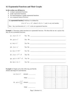
4 Transformations of Monomials: When graphing certain Polynomial Functions , we can use the Graphs of monomials we already know, and transform them using the techniques we learned earlier. Example 1: Sketch the graph of the function ()32 Pxx= +n by transforming the graph of an appropriate function of the form yx=. Indicate all x- and y-intercepts on the graph . Solution: Based on the transformation techniques, we know the graph of is the reflection of the graph of ()32 Pxx= +3yx= in the x-axis, shifted vertically up 2 units. Thus, Most Polynomial Functions cannot be graphed using transformations though.

5 For instance in the Polynomial function ()3252 Rxxx1= +, By: Crystal Hull we cannot determine easily what function s graph we should perform transformations on to graph ()Rx. Therefore, we will need a new method for finding the Graphs of more complex polynomials . End Behavior of polynomials : The end behavior of a Polynomial is a description of what happens as x becomes large in the positive or negative direction. To describe end behavior, we use the following notation: x means x becomes large in the positive direction x means x becomes large in the negative direction For example, the monomial 3yx= has the end behavior y as x and y as x The end behavior of a Polynomial graph is determined by the term of highest degree.

6 For instance, the Polynomial has the same end behavior as ()5234fxxx= +2()53fxx= because both are polynomials of degree 5. By: Crystal Hull Example 2: Determine the end behavior of the Polynomial ()64642 Qxxxx3= + . Solution: Since Q has even degree and positive leading coefficient, it has the following end behavior: y as x and as y x Using Zeros to graph polynomials : Definition: If is a Polynomial and c is a number such that , then we say that c is a zero of P. The following are equivalent ways of saying the same thing. P()0Pc= 1. c is a zero of P 2. xc= is a root of the equation ()0Px= 3.

7 Xc is a factor of ()Px When graphing a Polynomial , we want to find the roots of the Polynomial equation . To do this, we factor the Polynomial and then use the Zero-Product Property (Section ). Remember that if ()0Px=()0Pc=, then the graph of ()yPx= has an x-intercept at xc=, so the x-intercepts of the graph are the zeros of the function. Example 3: Find the zeros of the Polynomial ()271Rx xx2= +. Solution: Step 1: First we must factor R to get ()()()43 Rxxx= Step 2: Since 4x is a factor of ()2712Rx xx= +, 4 is a zero of R, and since 3x is a factor of ()Rx2712xx= +, 3 is a zero of R. The following theorem and its consequences will be used to help us graph polynomials .

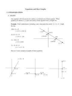
8 Intermediate Value Theorem for polynomials : If P is a Polynomial function and ()Pa and ()Pb have opposite signs, then there exists at least one value c between a and b for which . ()0Pc= The figure below graphically demonstrates this theorem. By: Crystal Hull One important consequence of this theorem is that between any two successive zeros, the x-o, to sketch the graph of P, we first find all the zeros of P. Then we choose test points Guidelines for Graphing Polynomial Functions : 1. Zeros: Factor the Polynomial to find all its real zeros; these are the . Test Points: Make a table of values for the Polynomial .

9 Include test ow . End Behavior: Determine the end behavior of the Polynomial .. graph : Plot the intercepts and other points you found in the table. values of a Polynomial are either all positive or all negative. That is, between two successive zeros the graph of a Polynomial lies entirely above or entirely below theaxis. Sbetween (and to the right and left of) successive zeros to determine whether ()Px is positive or negative on each interval determined by the zeros. x-intercepts of the graph . 2points to determine whether the graph of the Polynomial lies above or belthe x-axis on the intervals determined by the zeros.

10 Include the y-intercept in the table 3 4 Sketch a smooth curve that passes through these points and exhibits the required end behavior. By: Crystal Hull Example 4: Sketch the graph of the function . Make sure your graph shows all intercepts and exhibits the proper end behavior. () ( )( )212 Pxxx=+ Solution: Step 1: First we must find all the real zeros of ()Px. Since is already factored, it is easy to see () ( )( )212 Pxxx=+ the zeros are 1x= and 2x=. Therefore, the x-intercepts are and 1x= 2x=. Step 2: Now we will make a table of values of ()Px, making sure we choose test points between (and to the left and right of ) successive zeros, and include the y-intercept.