Transcription of Quantification using Asymmetric Line-Shapes - …
1 Copyright 2005 Casa Software Ltd Quantification using Asymmetric Line-Shapes While the following discussion centres on a Doniach-Sunjic (DS) line-shape, the issues discussed are also important for all Asymmetric Line-Shapes . Asymmetry is often encountered in synchrotron and XPS data; the desire to use appropriate Line-Shapes is understandable, however when the intention is to use the intensities measured using the area of an Asymmetric peak as part of a Quantification procedure the drawbacks of Asymmetric Line-Shapes should be understood. The fundamental problem with Asymmetric Line-Shapes is that the functional forms for these Line-Shapes are ill-defined in terms of area. For example, the theoretically based DS line- shape, when integrated between plus and minus infinite is, in general, infinite. This is in contrast to the Gaussian and Lorentzian Line-Shapes , both of which when integrated from plus and minus infinite are finite.
2 The consequence of the infinite area beneath a DS. curve is that the area measured by such a curve is quite arbitrary and can be chosen to be any value one desires. One response to the infinite area beneath a DS curve is to assume the area is determined by integrating the line-shape over the limits defined by a Quantification region. The problem with this approach is that small adjustments to the asymmetry parameter or full- width-half-maximum (FWHM) will influence the intensity of the DS peak and what is worse, the area becomes dependent on the users choice for the limits of the Quantification region and the measured intensity will depend on the location of the Asymmetric peaks within the region. While there is some justification for allowing the user to define the points at which the signal is deemed to be effectively zero (defined by the points at which the background meets the data), limiting a function that extends beyond these practical limits (with infinite intensity outside the region) is doubtful because the Quantification region limits effectively change the measured intensity from the line-shape without rhyme or reason.
3 A small practical change to the background limits will have unwelcome consequences for the DS peak area and therefore Quantification . An alternative strategy for dealing with the DS line-shape is to allow the data system to define the extent of the signal and then calibrate the measured intensity using adjustments to the relative sensitivity factors (RSF). The advantage of a fixed, but nevertheless arbitrary, interval over which the DS line-shape is integrated is that once the FWHM and asymmetry are established, the area beneath the chosen DS line-shape is defined and the measured area is determined by scaling the line-shape to the data. Doniach-Sunjic and Aluminium Metal:Oxide Ratio Consider the data in Figure 1. Metallic aluminium is measured using a DS line-shape to represent the Asymmetric nature of the Al 2p transition. Aluminium oxide is measured using a well-defined Gaussian-Lorentzian line-shape.
4 The tables in Figure 1 illustrate the problem of areas calculated using DS Line-Shapes . If the same RSF is applied to all three 1. Copyright 2005 Casa Software Ltd synthetic components and also the Quantification region, then the top Quantification table shows that the intensity measured from the component is different from the intensity measured by the Quantification region. The discrepancy in these measured areas is apparent from the fact that the ratio of the region area to the sum of the component areas is not 1:1; the area measured by the Quantification region is CPSeV while the sum of the three peaks yields an area of CPSeV. Figure 1: Region and each of the components are assigned the same value for the RSF. A useful indicator of a problem with the current Line-Shapes and RSF combination is the Effective RSF computed for the total data envelope. The value in Figure 2, displayed in the top-most text-field indicates an Effective RSF of , yet the RSF for each of the components is The Effective RSF is calculated from the uncorrected raw area from the Quantification region (version ) and the total RSF corrected area from the components (earlier version of CasaXPS use the component areas only to determine the Effective RSF).
5 If the RSF used for the region were applicable to each of the components in the model, then the Effective RSF would be equal to the RSF used in the region. The fact that the Effective RSF is not equal to the RSF used in the region means that the areas measured by the DS Line-Shapes are not directly comparable to the area of the Quantification region. The solution is to adjust the RSF in the metallic peaks modeled by the DS line-shape until the Effective RSF value is the intended RSF, namely, 2. Copyright 2005 Casa Software Ltd Figure 2: Component property page showing the Effective RSF in the top-most text-field. The Quantification table in Figure 3 corresponds to the adjusted RSF values for the DS. Line-Shapes . The value used for the RSF in the DS components depends on the DS. parameters and in this particular case, the RSF for the metallic components should be Provided the DS parameters remain fixed, the line-shape specific RSF will apply to other Al 2p spectra.
6 Interfering Species and Asymmetric Line-Shapes The use of the Effective RSF to monitor the suitability of an Asymmetric peak is a side- effect of the intended use for the Effective RSF. The primary purpose for the Effective RSF is for situations where a data envelope such as the one in Figure 4 is the result of two or more species. A peak-fit in which the distinct species are identified and assigned an individual RSF appropriate for each species provides a means of computing an 3. Copyright 2005 Casa Software Ltd average RSF for the combined set of peaks and species. The objective is to use this averaged RSF value when quantifying the sample using a lower resolution survey spectrum. While the atomic concentration for the overlapping peaks is not determined from the survey spectrum alone, without the effective RSF, the atomic concentrations for other non-overlapping peaks would be incorrect.
7 The full Quantification using the survey and the peak model for the overlapping peaks can proceed using the TAG mechanism in CasaXPS to proportion the intensity of the interfering species. Figure 3: Same data as in Figure 1, but with adjusted RSF for DS Line-Shapes . By way of a further example, consider the data in Figure 4. The model used to describe the underlying transitions includes two species and an Asymmetric line-shape is used to model the metal ruthenium doublet. The Quantification table annotating the spectrum assumes the metal and oxide peaks can be adjusted using the same RSF values for both symmetric and Asymmetric Line-Shapes . The Asymmetric line-shape, while accounting for the metallic peak shape requires calibrating. The problem is that the area beneath the data envelope must match the area measured by the sum of the peaks in the peak model. In this example, it is fortunate that there are only two identical Asymmetric peaks involved 4.
8 Copyright 2005 Casa Software Ltd and therefore the calibration for the Asymmetric peaks in the form of an adjusted RSF can be determined directly from the data. Figure 4: Asymmetric Line-Shapes constructed from the Gelius functional form. The adjustment to the RSF used in a Gaussian-Lorentzian peak should be computed from the raw area from the region together with the raw area from the individual components: RSF = RSF ( Aai ) /( Ar AGLi ). where, Ar is the raw area determined from the Quantification region, Aai is the raw area for peaks with the identical Asymmetric line-shape and AGLi is the raw area for the peaks with Gaussian-Lorentzian Line-Shapes . The raw areas for the spectrum in Figure 4 are displayed in Table 1. Computing the adjusted RSF for the Asymmetric peak changes the 5. Copyright 2005 Casa Software Ltd value used for the GL ruthenium peaks of to The new Quantification results are shown in Figure 5.
9 Raw Area Region Area Ru 3d5/2_a Ru 3d3/2_a C 1s_C-H C 1s_C-OH C 1s_C=O C 1s_O-C=O Ru 3d5/2_b Ru 3d3/2_b Table 1: Raw area values for the Quantification region and each of the components. Blue cells are the Asymmetric line-shape values. Figure 5: Quantification following the introduction of the adjusted RSF for the Asymmetric line- shapes. 6. Copyright 2005 Casa Software Ltd Calculating the adjusted RSF for the data in Figure 4 relies on the fact that a single Asymmetric line-shape is used to model both the metallic doublet peaks. The appropriate adjustments for Asymmetric peak RSFs may require the acquisition of data from a standard material to provide a known relationship between the peak areas; however this practice is also to be recommended for determination of the line-shape in the first place. Introducing asymmetry into a peak model based on the data envelope in Figure 4 would almost certainly introduce significant errors into the Quantification , since the highly correlated peaks are unlikely to provide an adequate description for the data without a rigid model and shape parameters such as asymmetry are certainly not rigid in nature.
10 Figure 6: Complex data envelope requiring DS line-shape and more. Trial and Error Approach to Adjusting RSF for Asymmetry Consider the data representing an As 3d complex in Figure 6. The DS-GL Line-Shapes in Figure 6 would be difficult to define simply using the given spectrum. The data is clearly a blend of multiple doublets, not all of which exhibit asymmetry and attempting to construct the peak model based on Figure 6 alone would be difficult. Fortunately, the sequence of data measured using a synchrotron (Beamline ALS, Berkeley CA) light- 7. Copyright 2005 Casa Software Ltd source (J. Thompson, PhD Thesis (2006), University of Salford, UK) also included a simple spectrum suitable for creating the shape of the Asymmetric doublet. The spectrum in Figure 7 not only allows the essential shape of the asymmetry to be assessed, but also a calibration for the Asymmetric peak area can a be made.