Transcription of Quantum Mechanics with Mathematica
1 Quantum Mechanics with MathematicaA tutorial for instructorsDaniel V. SchroederWeber State UniversityJuly 2019 IntroductionFor more than 20 years I have used Mathematica as a computational and visualizationtool when I teach Quantum Mechanics both at the upper-division level and in asophomore-level modern physics course. My goal in this tutorial is to help otherinstructors do the find Mathematica useful (in fact, almost indispensable) in these courses forseveral reasons: It allows students to quickly and easily plot any function, directly from itsformula, often with only a single line of code. With only a little more effort students can produce multidimensional plots,animated plots, and plots of complex-valued functions that use color hue torepresent phase.
2 Special functions such as hermite polynomials and spherical harmonics are builtinto Mathematica . Mathematica provides easy-to-use routines for numerical integration, solvingODEs, and diagonalizing matrices. Coding a PDE-solving algorithm is no harder in Mathematica than in any otherlanguage (although execution speed can sometimes be an issue).Because Mathematica makes so many computational and visualization tasks aboutas easy as they could possibly be, it frees students to think more about the physicsand less about the s main disadvantage is that it is a commercial and closed-sourceproduct, sold by Wolfram Research. The license fee can be a barrier to some stu-dents, and the secrecy of its internal algorithms can be a barrier to some , for most of the instructional uses I ll describe here, I don t know of asuitable is a versatile tool, and there are many ways to use it.
3 This tutorialincorporates my personal preferences, which include the following: We ll use Mathematica as a tool for graphics and numerical calculations, not (toany significant degree) for algebraic manipulations. This emphasis may comeas a surprise, because many people think of Mathematica primarily as algebraicmanipulation software. My personal opinion, based on many years of teachingexperience, is that Quantum Mechanics students should still do nearly all oftheir algebra by hand. I ll expect you to start with a blank window and type all of your Mathematicacode from scratch, so the code becomes your own. I expect the same of mystudents. Please resist the urge to copy-and-paste my code examples from an1 Neither Wolfram Research nor anybody else is paying me to say this. My only compensation fordeveloping this tutorial is my regular salary from Weber State University.
4 All opinions expressed inthis tutorial are my own, not those of WSU and certainly not those of Wolfram version of this document. Although Mathematica can be used toproduce canned simulations with code that is not meant to be read, I preferto empower students to use Mathematica as a tool, not a mere demonstration. In the code provided herein, I ve limited all variable names to use only charactersthat appear on the keyboard. Mathematica provides ways to enter Greek lettersand other special symbols, and can even be used as a mathematical typesettingtool. But typesetting is not our purpose here, and I want to provide codeexamples that are easy to type without hunting for GUI buttons or special keycombinations. Mathematica makes it possible to attach unit names to numerical quantities,but in this tutorial I will use natural units.
5 Typically this means setting~, theparticle mass, and some natural length or energy scale all equal to 1. Today sstudents find the use of natural units disorienting, because we have taughtthem in introductory physics to use SI units for everything. Nevertheless, bythe time they are learning Quantum Mechanics we need to teach them to usenatural units especially when they are doing computational work. Exerciseson converting between natural units and laboratory units are an important partof a Quantum Mechanics course, but are not part of this you would like to see how I have incorporated Mathematica calculations andvisualizations into the context of a Quantum Mechanics course for upper-divisionundergraduates, feel free to download my draft textbook, temporarily titledNoteson Quantum Mechanics , of the examples in this tutorial are taken from there, although I have triedto present them here in a way that s more efficient for someone who already knowsquantum Mechanics .
6 Even if that textbook isn t appropriate for the style or level ofyour own course, I hope you will find some useful examples in this tutorial, and thatyour students will gain a better understanding of Quantum Mechanics through theuse of tutorial is organized into two major sections: Visualization and Basic plots and basic syntaxThere s no better first exercise with Mathematica than making a basic plot, of areal-valued function of a single variable. Here s an example, for a harmonic oscillatoreigenfunction:Plot[(4x^4 - 12x^2 + 3)Exp[-x^2/2], {x, -5, 5}]Type this line into Mathematica now, then hit shift-enter to execute it. The plotshould appear in a single line of code illustrates several of Mathematica s most important fea-tures:3 Mathematica code is built out offunctions, such asPlotandExp.
7 Functionnames are case-sensitive, and all of Mathematica s built-in function names beginwith capital letters. Function arguments are enclosed in square brackets and separated by thePlotfunction has two arguments (both compound structures), whiletheExpfunction has just one. The first argument ofPlotis a mathematical expression, built out of theExpfunction and the operators+,-,/, and^. Multiplication requires no operator(just as in standard math notation), although you can always use*for clarity.(In a product of two variables such asaandbyou need to writea*bora b, soMathematica won t think you re referring to a single variable namedab.) In compound math expressions, exponentiation takes precedence over multipli-cation and division, which in turn take precedence over addition and subtrac-tion. So-x^2/2means (x2)/2, not x2/2.
8 To override the default groupingyou can use parentheses. The spaces that I ve inserted around the+and-aremerely for readability. The second argument ofPlotis alist, delimited by curly braces, with the threeelements of the list separated by commas. Here the list specifies the independentvariable of the function to plot, followed by the starting and ending values ofthis variable. I ll say more about lists namesFor all but the simplest tasks, you ll want to break up your Mathematica code intomultiple statements, to be executed in sequence. The following three lines producethe same output as the single line above, but provide more flexibility:psi = (4x^4 - 12x^2 + 3)Exp[-x^2/2];xMax = 5;Plot[psi, {x, -xMax, xMax}]Here I ve assigned the namespsiandxMaxto the function I want to plot and themaximumxvalue, so I can more easily modify or reuse these quantities.
9 The semi-colons serve as statement separators, and also suppress any displayed output of thelines that precede them. Go ahead and test this code now, putting all three linesinto a single Mathematica cell (as indicated by the bracket at the window s rightmargin). Again hit shift-enter to execute the code. Then try modifyingxMax, andpsitoo if you wish, to see how the plot all of Mathematica s built-in names (such asPlotandExp) begin withcapital letters, it s a good habit to begin all your own names (such aspsiandxMax) with lower-case letters. Then you can easily tell at a glance which names areMathematica s and which are yours. You ll also avoid inadvertent name conflicts,without having to learn all of Mathematica s built-in names (about 5000 of them, asof this writing).
10 4 Plot optionsIf you setxMaxtoo high in the previous example, you ll notice that Mathemat-ica expands the vertical scale of the plot and clips off the peaks of the function sfive bumps. This is because Mathematica thinks you want to see more detail inthe small function values that occur at larger values of|x|. To override this often-unwanted behavior, you can use thePlotRangeoption:xMax = 12;Plot[psi, {x, -xMax, xMax}, PlotRange->All]Try this modification now, then try providing an explicit range for the plot, using atwo-element list:PlotRange->{-5, 5}Here are a couple of other useful options for modifying the appearance of aPlot:Plot[psi, {x, -xMax, xMax}, PlotStyle->{Blue, Thick},AspectRatio-> ]You can specify options in any order, always separated by commas. For a complete listof options to use withPlot, use the menus to find the Mathematica documentation( Help Wolfram Documentation in my version), then use the search feature tofind thePlotfunction and, on its documentation page, scroll down to the Options of the colorBlue, you can (of course) specify other pre-defined colors, ordefine your own colors using eitherHueorRGBC olor:Hue[ , 1, 1]RGBC olor[ , 0, 1]Try each of these, varying the numerical values to see how the color changes.