Transcription of Plotting functions of more than one variable with Mathematica
1 Plotting functions of more than one variablewith MathematicaPhysics 3510, Weber State UniversityThis tutorial assumes that you are already somewhat familiar with Mathematica . So, forexample, you should know how to express basic arithmetic operations, and understand thedifference between parentheses(), square brackets[], and curly braces{}, and rememberthat the names of variables and functions are case-sensitive, but the names of all built-infunctions start with capital should also already know how to plot a simple function of one variable , for example,Plot[x^3-2x, {x, -2, 2}, PlotRange->{-3, 3}, PlotStyle->{Red, Thick}]where{x, -2, 2}is a common list construction that means (in this context) for values ofxranging from 2 to 2, whilePlotRangeandPlotStyleare two of the many options thatcan modify the appearance of the plot.
2 Please type this instruction into Mathematica now, towarm up your fingers and make sure that your Mathematica system is working. Rememberthat you need to use shift-enter to send the instruction to the Mathematica functions of two variablesOur main goal in this tutorial is to explore ways to plot functions oftwovariables. An exampleof such a function, which we ll work with for a while, isf = (x+y)^3 - 8(x+y) - 2(x-y)^2where I ve given the function a name,f, because we ll be using it repeatedly. Again, pleaseenter this line into most basic way of Plotting a function of two variables isDensityPlot:DensityPlot[f, {x, -2, 2}, {y, -2, 2}]After you enter this instruction, you should see a square-shaped plot with the first variable (herex) along the horizontal axis and the second variable (herey) along the vertical the function are represented by colors.
3 Which colors correspond to the lowestfunction values, and which correspond to the highest?Just as withPlot, there are many options you can use to modify the output try the optionColorFunction->"SunsetColors"and see how you like the new colorscheme. To see a list of all the built-in color schemes, open a documentation window ( Wol-fram Documentation under the Help menu in my version) and search for color schemes .Try a couple of other color functions in yourDensityPlotand see how you like them. Youcan also create your own color functions by saying something like this:ColorFunction -> Function[Blend[{Black, Blue, White}, #]]Try it! (The symbol#signifies the argument of the function; feel free to look up purefunctions andBlendin the documentation if you re curious about how exactly this syntaxworks.)
4 If you re not satisfied with blends of named colors likeBlue, you can define your owncolor usingRGBC olor[r, g, b], where each of the three arguments is a number between 0and 1, for example,RGBC olor[.5, 0, 1].1 Another common way to visualize a function of two variables is with contour lines, whichconnect points that have the same function value as on a topographic map. Try changingDensityPlottoContourPlotin the previous example, and notice that in addition to thecontour lines you still get the colors, but they now go in steps at the contour lines insteadof varying smoothly. Also notice that if you hover the mouse cursor over a contour line, youget a little popup note that tells you the function value on that contour.
5 Try the optionContours->30to increase the number of third way of Plotting a function of two variables is with a surface plot, where the functionvalue is plotted on a third axis in three dimensions:Plot3D[f, {x, -2, 2}, {y, -2, 2}]To view the surface from different directions, just drag it with the mouse. You can againuse theColorFunctionoption to change the colors, but to apply a homemade Blendto thefunction values you need to change#to#3in the syntax given above. Notice that the colors aremodified by simulated lighting that illuminates the surface from certain directions (which youcan also change if you wish). Another useful option for surface plots isBoxRatios->{1,1,1}(which you should now try).
6 Vector functions in two dimensionsSo much forscalar-valued functions of two variables; now what about a function (often calleda field ) whose value at any point is avector?Although we could start over and define each component of a vector field from scratch, wecan also make a vector field by taking the gradient of our scalar function:vx = D[f, x]vy = D[f, y]This is Mathematica s notation for partial derivatives. ( Mathematica actually providesGrad,Div, andCurlfunctions, but they re not worth the trouble when you re working in Cartesiancoordinates.)To plot a two-dimensional vector field, useVectorPlot:VectorPlot[{vx, vy}, {x, -2, 2}, {y, -2, 2}]This evaluates the vector field at points on a rectangular grid, and draws an appropriate arrowcentered on each grid point.
7 To change the grid resolution, use theVectorPointsoption:VectorPoints -> {20, 20}Of course there s also an option to change the colors of the arrows:VectorColorFunction -> Function[Green](This pure function simply assigns the colorGreento all vectors; if you want to get fancy, youcan assign colors based on the vectors components or lengths or locations.)VectorPlotscales the lengths of the arrows automatically. Often you ll want to omit afew of the biggest vectors from the plot, in order to enlarge the rest of them. You can do thiswith theVectorScaleoption:VectorScale -> {Automatic, Automatic, Function[If[#5>40, 0, #5]]}2 Here40is the cutoff applied to the vector magnitudes. Try some other values of this cutoff,and also try replacing the firstAutomaticwith a number ; this is the maximum size atwhich the vectors are drawn, in units of the full size of the plot.
8 If you want to fully understandVectorScale, look it up in the you might want to overlay a vector plot on a density or contour plot of a relatedscalar function. While Mathematica does provide a combinedVectorDensityPlotfunction,you ll have more control if you create the two plots separately and then combine them usingShow. For example:cplot = ContourPlot[f, {x, -2, 2}, {y, -2, 2}];vplot = VectorPlot[{vx, vy}, {x, -2, 2}, {y, -2, 2}];Show[cplot, vplot]Notice that I ve given names to the two individual plots so I can refer to them in the thirdline. Please try this example and then dress it up using several of the options described of three variablesVisualizing a function of three variables is considerably harder, because there s no perfect wayto prevent the stuff in front from obscuring your view of the stuff in back.
9 Mathematicaonly recently added aDensityPlot3 Dfunction, and so far I haven t managed to get it to givedecent also provides aContourPlot3 Dfunction for three-dimensional contour plots,as well as aVectorPlot3 Dfunction for 3-D vector plots. Both of these plot types workbest on functions (fields) that are large within some central region, dying out with , many examples in electromagnetism have that than trying to describe all the options and pitfalls of these 3-D plots in detail, I lljust give you the following example to try out:f3 = 1/Sqrt[x^2 + y^2 + (z-1)^2] + 1/Sqrt[x^2 + y^2 + (z+1)^2]ContourPlot3D[{f3== , f3==2, f3== , f3==3},{x, -2, 2}, {y, -2, 2}, {z, -2, 2},Mesh->None, ContourStyle->Directive[Opacity[ ]]]v3x = D[f3, x]; v3y = D[f3, y]; v3z = D[f3, z].
10 VectorPlot3D[{v3x, v3y, v3z}, {x, -2, 2}, {y, -2, 2}, {z, -2, 2}]Try modifying this example to see the effects of the various choices I ve made, and use thedocumentation to learn 3-D visualization is inherently difficult, a better approach is often to view justone two-dimensional slice at a time, using the various 2-D visualization techniques describedabove. So I ll leave you with this final, quick example to try:slice = f3 /. y -> 0 ContourPlot[slice, {x, -2, 2}, {z, -2, 2}]And with that, I hope you now feel ready to plot and visualize the functions and fields thatwe will encounter in electromagnetic