Transcription of Results from the Dixit/Stiglitz monopolistic …
1 Results from the dixit /Stiglitzmonopolistic competition modelRichard FoltynFebruary 4, 2012 Contents1 Introduction12 Constant elasticity sub-utility Preferences and demand .. case .. case ( dixit - stiglitz lite ) .. Firms and production .. Market equilibrium ..81 IntroductionThe Dixit/Stiglitz monopolistic competition model has been widely adopted in various fieldsof economic research such as international trade. The dixit and stiglitz (1977) paper actuallycontains three distinct models, yet economic literature has mostly taken up only the first one(constant elasticity case) and its market equilibrium solution. The main Results of this subsetof dixit and stiglitz (1977) are derived and explained below in order to aid in understandingthis widespread Constant elasticity sub-utility Preferences and demandAssumption are given by a (weakly-)separable, convex utility functionu=U(x0,V(x1,x2.))
2 ,xn))whereU( ) is either a social indifference curve or the multiple of a representative consumer a numeraire good produced in one sector whilex1,x2,..,xnare differentiatedgoods produced in another weakly-separable utility functions, the MRS (and thus the elasticity of substitution) of two goodsfrom the same group is independent of the quantities of goods in other sub-groups (see Gravelle and Rees2004, 67).1 dixit and stiglitz (1977) treat three different cases in which they alternately impose two ofthe three following restrictions:1. symmetry ofV( ) to its arguments;2. CES specification forV( )3. Cobb-Douglas form forU( )However, throughout the literature many authors have imposed all three restrictions togetherin what Neary (2004) calls dixit - stiglitz lite.
3 The next section examines the more general case in which only restrictions 1 and 2 areimposed. Subsection briefly looks and the more special case of dixit - stiglitz lite . General caseFirst-stage the CES case the utility function is given asu=U x0,[ ix i]1/ with (0,1) to allow for zero quantities and ensure concavity ofU( ). is called thesubstitution or love-of-variety ,U( ) is assumed to behomotheticin its ( ) is a separable utility function, the consumer optimization problem can be solvedin two separate steps: first the optimal allocation of income for each subgroup is determined,then the quantities within each a quantity index presenting all goodsx1,x2.
4 ,xnfrom thesecond sector such thaty [ ix i]1/ .(1)Figure 1 shows some illustrative examples for the two-dimensional case. As required, theutility function is concave andx1,x2are neither complements nor perfect substitutes if (0,1).The first-stage optimization problem is given as follows:max. U(x0,y) +q y=IwhereIis the income in terms of the numeraire andqis the price index = 1,x1,..,xnare perfect substitutes as the subutility function simplifies toV(x1,x2,..,xn) = ixiand thus it does not matter whichxiis consumed. For <0 they are complements (see Brakmanet al. 2001, 68).3 The income consists of an initial endowment which is normalized at 1, plus firm profits distributed toconsumers or minus a lump sum required to cover firm losses.
5 However, since the discussion here islimited to the market equilibrium case, firms make zero profit soI= 1:CES functions with two-dimensional domain and varying parameter (from left to right: ={-10, , }). The first case is excluded in this model due to the restrictions on parameter .From the LagrangianL=U(x0,y) [x0 qy I] we obtain the first-order conditions L x0=U0 = 0(2) L y=Uy q= 0(3) L =x0+qy I= 0 From (2) and (3) we get the necessary conditionUyU0=q=pyp0(4)which is the familiarUi/Uj=pi/pjasqis the price index foryandp0= 1 due to thenumeraire definition. SinceU( ) was assumed homothetic, this uniquely identifies the shareof expenditure forx0andybecause these solely depend on relative marginal utilities.
6 Denotethe share of expenditure onyass(q) and that onx0as (1 s(q)). Then the optimal quantitiesfor each sector arex0= (1 s(q))Iy=s(q)Iq(5)Second-stage the definition ofyands(q), the second-state problemismax. y=[ ix i]1/ ipixi=s(q)I3 The LagrangianL= ( ix i)1/ ( ipixi s(q)I) yields the first-order conditions L xi=y1 x 1i pi= 0(6) L = ipixi s(q)I= 0(7)Solving (6) forxigivesxi=y( pi)1/( 1)(8)Inserting this into (7) and solving for we get ipiy( pi)1/( 1)=s(q)I 1/( 1)y ip /( 1)i=s(q)I 1/( 1)=s(q)I)y[ ip /( 1)i] 1(9)Finally, plugging (9) back into (8) we get the preliminary demand function facing a singlefirm in the second sector:4xi=s(q)Ip1/( 1)i jp /( 1)j 1(10)To further simplify this expression, take (10) to the power of and sum overi.
7 5x i= (s(q)I) p /( 1)i jp /( 1)j ix i= jp /( 1)j (s(q)I) ip /( 1)iy=[ ix i]1/ = jp /( 1)j 1s(q)I[ ip /( 1)i]1/ y=s(q)I[ ip /( 1)i]( 1)/ (11)From (5) and (11) we obtainResult the utility function given in Assumption and the composite quantityindex from Definition the correspondingprice indexisq=[ ip /( 1)i]( 1)/ (12)4 The summation index has been changed tojto reflect that it in is unrelated last step follows from the fact that both sums are identical, regardless whether the Result , (10) can be simplified to arrive atResult the utility function given in Assumption , the resultingdemand functionfacing a single firm isxi=y[qpi]1/(1 )(13)withyandqdefined in (1) and (12), remarks regarding the demand function and CES preferences are in , by pluggingy=s(q)I/qinto (13) and taking logs, it can easily be seen that thevarietiesx1,x2.
8 ,xnhave unitincome elasticities logxi/ , assuming a sufficiently large number of varieties so that pricing decisions of a singlefirm do not affect the general price index, theprice elasticity of demandforxiis d= logxi logpi 1(14)At this point it is convenient to define 1/(1 ) so that d= .6 Third, to get theelasticity of substitutionbetween two varieties, from (6) we see thatxixj=[pjpi]1/(1 )and hence the elasticity of substitution can be obtained as s= log(xj/xi) log(pi/pj)= log(pi/pj)1/(1 ) log(pi/pj)=11 = (15)This can be summarized asResult preferences given in Assumption result inconstantdemandand substitution elasticities given by d=1 1= s=11 = Often the model is specified directly in terms of instead of ,7withu=U(x0,y), y [ ix1 1/ i]1/(1 1/ ), q [ ip1 i]1/(1 )
9 Fourth, to see why the CES utility specification is called variety-loving , inspect the large-subgroup case with many varietiesnwith similar price levels, pand hencexi= expenditure is equally divided over all varietiesx1,x2,..,xnsince they symmetrically6 Here is different from (q) in dixit and stiglitz (1977), but reflects the notation of many other dixit - stiglitz -based example, see Baldwin et al. (2005, 38).5enter into the subutility function. If there existnvarieties, the expressions foryandqsimplify toy=[n ix ]1/ =xn1/ (16)q=[n ip /( 1)]( 1)/ =pn( 1)/ (17)Plugging (5) and (17) into (13) gives a simplified demand function for the large-subgroupcase:x=s(q)Inp.(18)Substit uting this forxin the subutility function (1), we obtainV(n) =y=[n i[s(q)Inp] ]1/ =n(1/ )s(q)Inp=n1/ 1(nx)which is increasing innas (0,1) by assumption.
10 The last equality provides some intuitiveinsights: since (nx) is the actual quantity produced, the termn1/ 1>1 can be seen asan additional bonus , so variety represents an externality or the extent of the the market sizenxhas a more than proportional effect on utility due to this term(Brakman et al. 2001, 68).That utility increases with variety can also be seen by recalling thatV(x) =y=s(q)I/qand examining howqfrom (17) changes withn, as shown in Figure 2:Price indexqas a function of the number of varietiesn(assumingp= 1) = = = is evident that for constant expenditure, the price index falls rapidly, with utility risingas a consequence. This effect is more pronounced for closer to 0, which can intuitivelybe explained using Figure 1: for close to 1, all varieties are close substitutes and henceintroducing another similar variety only moderately increases utility.