Section 1.0 : Introduction - Quarter Wave

1 Section : Introduction By Martin J. King, 07/05/02 Copyright 2002 by Martin J. King. All Rights Reserved. Page 1 of 5 Section : Introduction Over the years, many articles have appeared in Speaker Builder (now audioXPRESS) presenting test data and theories related to transmission line loudspeaker behavior. In the issues following each article, letters to the editor have debated the merits of the author s results. Some of these articles have been heatedly discussed over the Internet without any consensus of opinion being reached. Transmission line designs elicit strong differing opinions that seem to be largely based on personal experience or vague design guidelines, rules of thumb, that are quoted as fact without any specific reference source being provided.

2 There does not appear to be a generally accepted transmission line mathematical model, similar to the closed and ported box models, where one can give the numerical values of several key parameters and uniquely define the configuration being discussed. Over ten years ago, I heard my first transmission line system at the home of a local audio club member. The quality of the bass reproduction was impressive and my interest in this exotic enclosure was stimulated. Since then I have read most of the technical literature on the design of transmission lines, followed the frequent discussions on several e-mail lists and bulletin boards, and visited a number of websites devoted to this type of enclosure design. After many years of reading and thinking about transmission lines, I decided three years ago, that it was time to build another set of speakers and that I was going to seriously consider a transmission line system.

3 Since there was no acceptable design method available, my first step in exploring the transmission line s acoustic potential was to write the necessary design software and correlate it against test results. I had already designed and built several sealed and ported speaker systems based on the lumped parameter circuit models used in the classic papers by Thiele(1) and Small(2-4). For each of these designs, I wrote my own software using the MathCad(5) computer program. For me, formulating and solving the computer simulation of a speaker system is as interesting and challenging as the construction of the speaker system itself. After the speaker construction is completed, measuring and achieving good correlation with the mathematical predictions is extremely rewarding.

4 Hopefully, a well-designed speaker system that measures as predicted also sounds right. So I started the transmission line project by putting a MathCad computer model together using equations from the articles I had collected and studied. Before I go any further, I want to introduce my definition of a transmission line loudspeaker. I define a transmission line loudspeaker as a driver mated to a resonant tube where the natural frequencies and mode shapes of the air in the tube are used to tailor the total system response. This definition does not include any restrictions on the location of the driver in the tube or the boundary conditions at either end of the tube. Also, this definition does not place any requirement on the amount or type of fiber stuffing material that may be placed inside the tube to attenuate the standing waves associated with the tube s natural frequencies.

5 This is a very broad definition. What follows is my design method for a Quarter wave length transmission line with a closed end and an open end, or terminus, which emits sound that contributes to the system response over the bass frequency range. Section : Introduction By Martin J. King, 07/05/02 Copyright 2002 by Martin J. King. All Rights Reserved. Page 2 of 5 First Transmission Line Computer Models : The first mathematical model formulated took the equivalent circuits used by Thiele and Small and replaced the circuit elements modeling the boxes with a transmission line acoustic or electrical impedance. Figure shows the acoustic equivalent circuit, using the impedance analogy, while Figure shows the electrical equivalent circuit.

6 An excellent discussion of this kind of equivalent circuit modeling can be found in the referenced acoustics text by Beranak(6). I am assuming that everybody is familiar with the Thiele / Small parameters for a driver or that you can read the references to bring yourself up to speed. All of the circuit elements in Figure and can be derived from the Thiele / Small driver parameters, as shown in the figures, except the equivalent electrical impedance Zel and the equivalent acoustic impedance Zal of the transmission line. Expressions for the transmission line electrical and acoustic impedance are required to completely solve each of the circuits. My first mathematical models were based on Bradbury s(8) paper published by the Audio Engineering Society.

7 In his paper, Bradbury presents an elegant derivation of the wave equation applied to sound waves passing through a fibrous tangle. At low frequencies, the air and the fibers are coupled by a viscous damping coefficient that drags the fibers along with the air. As sound waves pass through the fibrous tangle, the waves are attenuated and the speed of sound is significantly reduced due to the added mass of the moving fibers. As the frequency of the sound wave increases, this coupling decreases and a transition is made to a stationary fibrous tangle that only attenuates the sound waves without any reduction in the speed of sound. This particular model of sound waves passing through a fibrous tangle is very popular and I have seen a number of attempts to apply it to the analysis of transmission line enclosures.

8 I spent a long time deriving and experimenting with Bradbury s equations. From this effort, I extracted an expression for the acoustic impedance of the transmission line, as seen by the driver, and an expression for the velocity of the air at the open end, or terminus, as a function of the driver velocity. Bradbury s equations are for a constant cross- Section transmission line with constant stuffing density. The acoustic impedance was inserted into the equivalent circuits shown in Figures and After solving the acoustic equivalent circuit in Figure for Ud, the air velocity at the terminus can be calculated as shown in the last four equations at the bottom of the figure. Using the velocities of the driver and the air at the terminus, the sound pressure for each can also be calculated.

9 These two sound pressures can then be summed, taking into account the relative phase angle, and the total system sound pressure level SPL and phase plotted. There were two sources of data available to me for correlating this model. Bullock and Hillman(9) wrote a paper in 1986 that used Bradbury s equations to model a test transmission line. A second source for data was a contact I made over the Internet. My electronic contact was kind enough to provide a number of measurements for several transmission line and driver combinations. We compared my computer model predictions against his test data. For both sets of results, the correlation showed promise but was clearly not accurate enough to design an enclosure. The general shapes of the impedance and SPL response plots were close but the locations of the peaks and valleys were shifted in frequency.

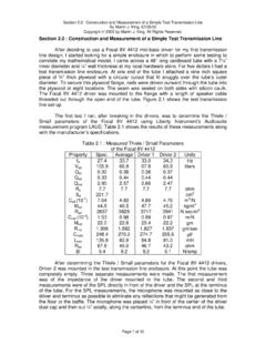
10 This was particularly evident in the frequency range below 200 Hz. Section : Introduction By Martin J. King, 07/05/02 Copyright 2002 by Martin J. King. All Rights Reserved. Page 3 of 5 Although the computer model, based on Bradbury s equations, did not correlate as well as I would have liked, I saw enough potential to build my own test line and start formulating a new mathematical model. My goal at this point in the project was to derive and correlate a better mathematical model and use it to design a transmission line system. The next step was to select a driver and fabricate a simple transmission line for testing and measurement. Before I could start testing, I needed to select and purchase a mid-bass driver. Since I wanted to eventually build a two-way system for my first transmission line project, I researched six and eight inch diameter mid-bass drivers from several highly rated manufacturers.