Transcription of Section 16: Magnetic properties of materials (continued)
1 Physics 927 1 Section 16: Magnetic properties of materials (continued) Ferromagnetism Ferromagnetism is the phenomenon of spontaneous magnetization the magnetization exists in the ferromagnetic material in the absence of applied Magnetic field. The best-known examples of ferromagnets are the transition metals Fe, Co, and Ni, but other elements and alloys involving transition or rare-earth elements also show ferromagnetism. Thus the rare-earth metals Gd, Dy, and the insulating transition metal oxide CrO2 all become ferromagnetic under suitable circumstances. Ferromagnetism involves the alignment of an appreciable fraction of the molecular Magnetic moments in some favorable direction in the crystal. The fact that the phenomenon is restricted to transition and rare-earth elements indicates that it is related to the unfilled 3d and 4f shells in these substances. Ferromagnetism appears only below a certain temperature, which is known as the ferromagnetic transition temperature or simply as the Curie temperature.
2 This temperature depends on the substance, but its order of magnitude is about 1000 K for Fe, Co, Gd, Dy. It might be however much less. For example it is 70K for EuO and even less for EuS. Thus the ferromagnetic range often includes the whole of the usual temperature region. Above the Curie temperature, the moments are oriented randomly, resulting in a zero net magnetization. In this region the substance is paramagnetic, and its susceptibility is given by CCTT = (1) which is the Curie-Weiss law. The constant C is called the Curie constant and TC is the Curie temperature. The Curie-Weiss law can be derived using arguments proposed by Weiss. In the ferromagnetic materials the moments are magnetized spontaneously, which implies the presence of an internal field to produce this magnetization. Weiss assumed that this field is proportional to the magnetization, E =BM (2) where is the Weiss constant.
3 Weiss called this field the molecular field and thought that this field results from all the molecules in the sample. In reality, the origin of this field is the exchange interaction. The exchange interaction is the consequence of the Pauli exclusion principle and the Coulomb interaction between electrons. Consider for example the system of two electrons. There are two possible arrangements for the spins of the electrons: either parallel or antiparallel. If they are parallel, the exclusion principle requires the electrons to remain far apart. If they are antiparallel, the electrons may come closer together and their wave functions overlap considerably. These two arrangements have different energies because, when the electrons are close together, the energy rises as a result of the large Coulomb repulsion. This is actually an explanation of the first Hund rule according to which the system of electrons tends to have a high possible spin, which is not forbidden by the Pauli principle.
4 As we see from this example the electrostatic energy of an electron system depends on the relative orientation of the spins: the difference in energy defines the Physics 927 2 exchange energy. The exchange interaction is short ranged. Therefore, only nearest neighbor atoms are responsible for producing the molecular field. The magnitude of the molecular (exchange) field is very large of the order of 107G or 103T. It is not possible to produce such field in laboratories. Weiss logic was as follows. Consider the paramagnetic phase: an applied Magnetic field B0 causes a finite magnetization. This in turn causes a finite exchange field BE. If P is the paramagnetic susceptibility, the induced magnetization is given by ()()00pEp =+=+MBBBM (3) Note that the magnetization is equal to a constant susceptibility times a field only if the fractional alignment is small: this is where the assumption enters that the specimen is in the paramagnetic phase.
5 Equation (3) should be considered as a self-consistent equation for the magnetization. It can be solved explicitly for the magnitude of the magnetization so that 01ppBM = (4) We know that the paramagnetic susceptibility is given by the Curie law P = C/T, where C is the Curie constant. We then find for the susceptibility of the ferromagnetic material 0 CMCCBTCTT === (5) The susceptibility (5) has a singularity at TC = C . At this temperature (and below) there exists a spontaneous magnetization, because if is infinite so that we can have a finite M for zero B0. Using the expression we obtained earlier for C, 223 BBNpCk =, the Curie temperature is given by 223 BCBNpTk =. (6) Reciprocal of the susceptibility per gram of nickel in the neighborhood of the Curie temperature (358 C). The dashed line is a linear extrapolation from high temperatures. Physics 927 3 The Curie-Weis law describes fairly well the observed susceptibility variation in the paramagnetic region above the Curie point ( ).
6 Only in the vicinity of the Curie temperature a notable deviations are observed. This due to the fact that strong fluctuations of the Magnetic moments close to the phase transition temperature can not be described by the mean field theory which was used for deriving the Curie-Weiss law. Accurate calculations predict that () (7) at temperatures very close to TC. We can also use the mean field approximation below the Curie temperature to find the magnetization as a function of temperature. We can proceed as before but instead of the Curie law which is valid for not too high Magnetic fields and not too low temperatures we can use the complete Brillouin function. If we omit the applied Magnetic field and replace B by the exchange field BE = M we find BBJgJMMNgJBkT = , (8) where ()JBx is the Brillouin function. This is a non-linear equation in M, which we can be solved numerically.
7 Now we shall see that solutions of this equation with nonzero M exist in the temperature range between 0 and TC. To solve (8) we write it in terms of the reduced magnetization BmNgJM = and the reduced temperature 222 BkTtNgJ =, whence JmmBt = (9) Graphical solution of Eq. (9) for the reduced magnetization m as a function of temperature. The left-hand side of Eq. (9) is plotted as a straight line m with unit slope. The right-hand side Eq. (9) is plotted vs. m for three different values of the reduced temperature t = kBT/N B2 = T/TC. The three curves correspond to the temperatures 2TC, TC,, and The curve for t = 2 intersects the straight line m only at m = 0, as appropriate for the paramagnetic region (there is no external applied Magnetic field). The curve for t = 1 (or T = TC) is tangent to the straight line m at the origin; this temperature marks the onset of ferromagnetism.
8 The curve for t = is in the ferromagnetic region and intersects the straight line m at about m = B,. As t 0 the intercept moves up to m = 1, so that all Magnetic moments are lined up at absolute zero. Physics 927 4 We then plot the right and left sides of this equation separately as functions of m, as in Fig. 2 which is plotted for J=S=1/2. The intercept of the two curves gives the value of m at the temperature of interest. The critical temperature is t = 1, or TC = N B2 /kB. The curves of M versus T obtained in this way reproduce roughly the features of the experimental results, as shown in Fig. 3 for nickel. As T increases the magnetization decreases smoothly to zero at T = TC. Saturation magnetization of nickel as a function of temperature, together with the theoretical curve for S = 1/2 on the mean field theory. The mean field theory does not give a good description of the variation of M at low temperatures.
9 The mean field theory predicts exponential convergence of the magnetization to the value at zero temperature. The experimental results show however a much more rapid dependence of M on temperature at low temperatures, namely 3 / 2 MATM = (10) where A is some constant different for different metals. The result (10) finds a natural explanation in terms of spin wave theory. Spin waves In ferromagnetic materials the lowest energy of the system occurs when all spins are parallel to each other in the direction of magnetization. When one of the spins is tilted or disturbed, however, it begins to precess due to the field from the other spins. Due to the exchange interaction between nearest neighbors the disturbance propagates as a wave through the system, as shown in A spin wave on a line of spins, (a) The spins viewed in perspective, (b) Spins viewed from above, showing one wavelength. The wave is drawn through the ends of the spin vectors.
10 Physics 927 5 Spin waves are analogous to lattice waves. In lattice waves, atoms oscillate around their equilibrium positions, and their displacements are correlated through lattice forces. In spin waves, the spins precess around the equilibrium magnetization and their precessions are correlated through exchange forces. Now we derive an expression for the frequency of the spin waves. We consider a linear chain of spins with nearest neighbor spins coupled by the Heisenberg interaction: 112 NpppUJ+== SS (11) where J is the exchange integral and Sp is spin at site p. For simplicity we will use classical theory in which spin operators are replaces by classical vectors. According to (11) the interaction which involves the p-th spin is ()112pppJ + +SSS. (12) This interaction can be rewritten as pp B, where pBpg = S is the Magnetic moment associated with spin Sp and pB is an effective Magnetic field or exchange field acting on this moment due to nearest neighbor spins: ()112pppBJg += +BSS.