Section 2.1 – Solving Linear Programming Problems

1 Math 1313 Page 1 of 19 Section Section Solving Linear Programming Problems There are times when we want to know the maximum or minimum value of a function, subject to certain conditions. An objective function is a Linear function in two or more variables that is to be optimized (maximized or minimized). Linear Programming Problems are applications of Linear inequalities, which were covered in Section A Linear Programming problem consists of an objective function to be optimized subject to a system of constraints.

2 The constraints are a system of Linear inequalities that represent certain restrictions in the problem. The Problems in this Section contain no more than two variables, and we will therefore be able to solve them graphically in the xy-plane. Recall that the solution set to a system of inequalities is the region that satisfies all inequalities in the system. In Linear Programming Problems , this region is called the feasible set, and it represents all possible solutions to the problem. Each vertex of the feasible set is known as a corner point.

3 The optimal solution is the point that maximizes or minimizes the objective function, and the optimal value is the maximum or minimum value of the function. The context of a problem determines whether we want to know the objective function s maximum or the minimum value. If a Linear Programming problem represents the amount of packaging material used by a company for their products, then a minimum amount of material would be desired. If a Linear Programming problem represents a company s profits, then a maximum amount of profit is desired.

4 In most of the examples in this Section , both the maximum and minimum will be found. Fundamental Theorem of Linear Programming To solve a Linear Programming problem, we first need to know the Fundamental Theorem of Linear Programming : Given that an optimal solution to a Linear Programming problem exists, it must occur at a vertex of the feasible set. If the optimal solution occurs at two adjacent vertices of the feasible set, then the Linear Programming problem has infinitely many solutions . Any point on the line segment joining the two vertices is also a solution.

5 Math 1313 Page 2 of 19 Section A graphical method for Solving Linear Programming Problems is outlined below. Solving Linear Programming Problems The Graphical Method 1. Graph the system of constraints. This will give the feasible set. 2. Find each vertex (corner point) of the feasible set. 3. Substitute each vertex into the objective function to determine which vertex optimizes the objective function. 4. State the solution to the problem. An unbounded set is a set that has no bound and continues indefinitely.

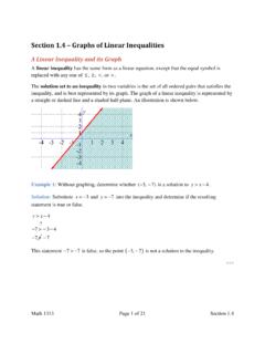
6 A Linear Programming problem with an unbounded set may or may not have an optimal solution, but if there is an optimal solution, it occurs at a corner point. A bounded set is a set that has a boundary around the feasible set. A Linear Programming problem with a bounded set always has an optimal solution. This means that a bounded set has a maximum value as well as a minimum value. Example 1: Given the objective function 103 Pxy= and the following feasible set, A. Find the maximum value and the point where the maximum occurs.

7 B. Find the minimum value and the point where the minimum occurs. Solution: We can see from the diagram that the feasible set is bounded, so this problem will have an optimal solution for the maximum as well as for the minimum. The vertices (corner points) of the feasible set are ()2, 2, ()3, 7, and ()5, 6. To find the optimal solutions at which the maximum and minimum occur, we substitute each corner point into the objective function, 103 Pxy= . Math 1313 Page 3 of 19 Section Vertex of Feasible Set Value of 103 Pxy= = = = ()2, 2 ()()10 23 214P= = ()3, 7 ()()10 33 79P= = ()5, 6 ()()10 53 632P= = We now look at our chart for the highest function value (the maximum) and the lowest function value (the minimum).

8 A. The maximum value is 32 and it occurs at the point ()5, 6. B. The minimum value is 9 and it occurs at the point ()3, 7. ** Example 2: Given the objective function 58 Dxy=+ and the following feasible set, A. Find the maximum value and the point where the maximum occurs. B. Find the minimum value and the point where the minimum occurs. Solution: We can see from the diagram that the feasible set is bounded, so this problem will have an optimal solution for the maximum as well as for the minimum.

9 The vertices (corner points) of the feasible set are ()0, 0, ()0, 3, ()1, 0, and ()2, 1. To find the optimal solutions at which the maximum and minimum occur, we substitute each corner point into the objective function, 58 Dxy=+. Math 1313 Page 4 of 19 Section Vertex of Feasible Set Value of 58 Dxy=+=+=+=+ ()0, 0 ()()5 08 00D=+= ()0, 3 ()()5 08 324D=+= ()1, 0 ()()5 18 05D=+= ()2, 1 ()()5 28 118D=+= We now look at our chart to find the maximum and the minimum of the objective function. A. The maximum value is 24 and it occurs at ()0, 3.

10 B. The minimum value is 0 and it occurs at ()0, 0. ** Example 3: Given the objective function 124 Cxy=+ and the following feasible set, A. Find the maximum value. B. Find the minimum value. Solution: Notice that the feasible set is unbounded. This means that there may or may not be an optimal solution which results in a maximum or minimum function value. The vertices (corner points) of the feasible set are ()0, 7, ()4, 2, and ()8, 0. We substitute each corner point into the objective function, as shown in the chart below.