Smith Chart - Amanogawa

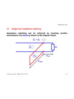
1 Transmission Lines Amanogawa , 2006 - Digital Maestro Series 165 Smith Chart The Smith Chart is one of the most useful graphical tools for high frequency circuit applications. The Chart provides a clever way to visualize complex functions and it continues to endure popularity, decades after its original conception. From a mathematical point of view, the Smith Chart is a 4-D representation of all possible complex impedances with respect to coordinates defined by the complex reflection coefficient. The domain of definition of the reflection coefficient for a loss-less line is a circle of unitary radius in the complex plane. This is also the domain of the Smith Chart .

2 In the case of a general lossy line, the reflection coefficient might have magnitude larger than one, due to the complex characteristic impedance, requiring an extended Smith Chart . Im( ) Re( )1 Transmission Lines Amanogawa , 2006 - Digital Maestro Series 166 The goal of the Smith Chart is to identify all possible impedances on the domain of existence of the reflection coefficient. To do so, we start from the general definition of line impedance (which is equally applicable to a load impedance when d=0) ()()()()01()1 VddZdZIdd+ == This provides the complex function ()(){}()Re,ImZdf= that we want to graph. It is obvious that the result would be applicable only to lines with exactly characteristic impedance Z0.

3 In order to obtain universal curves, we introduce the concept of normalized impedance ()()()01()1nZddzdZd+ == Transmission Lines Amanogawa , 2006 - Digital Maestro Series 167 The normalized impedance is represented on the Smith Chart by using families of curves that identify the normalized resistance r (real part) and the normalized reactance x (imaginary part) ()()()ReImnnnzdzjzrjx=+=+ Let s represent the reflection coefficient in terms of its coordinates ()()()ReImdj = + Now we can write ()()() ()() ()()()()()22221 ReIm1 ReIm1 ReIm2Im1 ReImjrjxjj+ + += + = + Transmission Lines Amanogawa , 2006 - Digital Maestro Series 168 The real part gives () ()()()()()()()()() ()()()()()()()( ) () ()()()()()()()2222222222222222221 ReIm1 ReIm11Re1Re1 ImIm01111Re1Re11Im1111Re 2Re1Im1111 ReIm11rrrrrrrrrrrrrrrrrrr = + + + + + =++ + ++ + =+++ + ++ =+++ + =++ = 0 Add a quantity equal to zero Equation of a circle Transmission Lines Amanogawa , 2006 - Digital Maestro Series 169 The imaginary part gives ()()()()()() ()()()()()()()()()()()()()

4 22222222222222222Im1 ReIm1 ReIm2Im11 02111 ReImIm2111 ReImIm11Re1 Imxxxxxxxxxxx = + + + = + += + + = + = =0 Multiply by xand add a quantity equal to zeroEquation of a circleTransmission Lines Amanogawa , 2006 - Digital Maestro Series 170 The result for the real part indicates that on the complex plane with coordinates (Re( ), Im( )) all the possible impedances with a given normalized resistance r are found on a circle with 1,011rrr ++ Center =Radius = As the normalized resistance r varies from 0 to , we obtain a family of circles completely contained inside the domain of the reflection coefficient | | 1 . Im( )Re( )r = 0r r = 1r = r = 5 Transmission Lines Amanogawa , 2006 - Digital Maestro Series 171 The result for the imaginary part indicates that on the complex plane with coordinates (Re( ), Im( )) all the possible impedances with a given normalized reactance x are found on a circle with 111,xx Center =Radius = As the normalized reactance x varies from - to , we obtain a family of arcs contained inside the domain of the reflection coefficient | | 1.

5 Im( )Re( )x = 0 x x = 1x = x = -1x = - Transmission Lines Amanogawa , 2006 - Digital Maestro Series 172 Basic Smith Chart techniques for loss-less transmission lines Given Z(d) Find (d) Given (d) Find Z(d) Given R and ZR Find (d) and Z(d) Given (d) and Z(d) Find R and ZR Find dmax and dmin (maximum and minimum locations for the voltage standing wave pattern) Find the Voltage Standing Wave Ratio (VSWR) Given Z(d) Find Y(d) Given Y(d) Find Z(d) Transmission Lines Amanogawa , 2006 - Digital Maestro Series 173 Given Z(d) Find (d) 1. Normalize the impedance ()()00 0ddnZRXzjrjxZZZ==+=+ 2. Find the circle of constant normalized resistance r 3.

6 Find the arc of constant normalized reactance x 4. The intersection of the two curves indicates the reflection coefficient in the complex plane. The Chart provides directly the magnitude and the phase angle of (d) Example: Find (d), given ()0d25100 with 50 ZjZ=+ = Transmission Lines Amanogawa , 2006 - Digital Maestro Series 174 1 -10 Normalization zn (d) = (25 + j 100)/50 = + j 2. Find normalized resistance circle r = 3. Find normalized reactance arc x = 4. This vector represents the reflection coefficient (d) = + | (d)| = (d) = rad = Lines Amanogawa , 2006 - Digital Maestro Series 175 Given (d) Find Z(d) 1.

7 Determine the complex point representing the given reflection coefficient (d) on the Chart . 2. Read the values of the normalized resistance r and of the normalized reactance x that correspond to the reflection coefficient point. 3. The normalized impedance is ()dnzrjx=+ and the actual impedance is ()()0000(d)dnZZzZrjxZrjZx==+=+ Transmission Lines Amanogawa , 2006 - Digital Maestro Series 176 Given R and ZR Find (d) and Z(d) NOTE: the magnitude of the reflection coefficient is constant along a loss-less transmission line terminated by a specified load, since ()()dexp2dRRj = = Therefore, on the complex plane, a circle with center at the origin and radius | R | represents all possible reflection coefficients found along the transmission line.

8 When the circle of constant magnitude of the reflection coefficient is drawn on the Smith Chart , one can determine the values of the line impedance at any location. The graphical step-by-step procedure is: 1. Identify the load reflection coefficient R and the normalized load impedance ZR on the Smith Chart . Transmission Lines Amanogawa , 2006 - Digital Maestro Series 1772. Draw the circle of constant reflection coefficient amplitude | (d)| =| R|. 3. Starting from the point representing the load, travel on the circle in the clockwise direction, by an angle 22d 2 d = = 4. The new location on the Chart corresponds to location d on the transmission line.

9 Here, the values of (d) and Z(d) can be read from the Chart as before. Example: Given 025100 50 RZjZ=+ = with find ()() = andfor Transmission Lines Amanogawa , 2006 - Digital Maestro Series 178 1 -10 -332-2 RzR R = 2 d = 2 (2 / ) = rad = z(d) (d) (d) = = j zn(d) = Z(d) = z(d) Z0 = Circle with constant | | Transmission Lines Amanogawa , 2006 - Digital Maestro Series 179 Given R and ZR Find dmax and dmin 1. Identify on the Smith Chart the load reflection coefficient R or the normalized load impedance ZR . 2. Draw the circle of constant reflection coefficient amplitude | (d)| =| R|.

10 The circle intersects the real axis of the reflection coefficient at two points which identify dmax (when (d) = Real positive) and dmin (when (d) = Real negative) 3. A commercial Smith Chart provides an outer graduation where the distances normalized to the wavelength can be read directly. The angles, between the vector R and the real axis, also provide a way to compute dmax and dmin . Example: Find dmax and dmin for 025100 ; 25100 (50)RRZj ZjZ=+ = = Transmission Lines Amanogawa , 2006 - Digital Maestro Series 180 1 -10 -332-2 RznR R2 dmin = dmin = 2 dmax = dmax = Im(ZR) > 0 Zj ZR=+=25100500 ()Transmission Lines Amanogawa , 2006 - Digital Maestro Series 181 1 -10 -2 RznR R2 dmin = dmin = 2 dmax = dmax = Im(ZR) < 0 Zj ZR= =25100500 ()Transmission Lines Amanogawa , 2006 - Digital Maestro Series 182 Given R and ZR Find the Voltage Standing Wave Ratio (VSWR)