Transcription of Stochastic Simulation - MIT
1 Spring 2024. Stochastic Simulation Cathy Wu Transportation: Foundations and Methods Wu 2. Readings 1. Larson, Richard C. and Amedeo R. Odoni. Urban Operations Research. Prentice-Hall (1981). Chapter 7: Simulations. URL. 2. (Optional) X. Wang et al., Traffic light optimization with low penetration rate vehicle trajectory data, Nat Commun, vol. 15, no. 1, Art. no. 1, Feb. 2024, doi: 45427-4. Wu 3. Unit 2: Queuing systems Modeling mathematical programs Uncertainty Linear programs Poisson process Sequential decision Queueing models problems Unit 2 LAB 1: Build your Time-space Cumulative Simplex method diagrams diagrams own traffic jam LAB 2: Build a queuing Vehicle Facility dynamics model for Seattle transit Markov chains dynamics Modeling Discrete event Markov decision processes Traffic flow Simulation Value iteration Numerical theory integration Stochastic Q-learning Integer programs Deep learning Branch-and-bound Deep Q Networks LAB 3: Build an AI agent LAB 4: Solve the traveling to optimize traffic salesman problem Wu Traffic light optimization with low penetration rate 4.
2 Vehicle trajectory data (Nature Communication, 2024). Overall result: Decreased the delay and number of stops at signalized intersections by up to 20% and 30% with data from as low as 6% vehicle penetration. Wu X. Wang et al., Traffic light optimization with low penetration rate vehicle trajectory data, Nat Commun, vol. 15, no. 1, Art. no. 1, Feb. 2024, doi: 5. Ideas from Unit 1+2. Time-space diagram Discrete event Simulation Newell's car following model G/D/1 queue Stochastic arrival process Probabilistic time-space (PTS). Bernoulli distribution! diagram X. Wang et al., Traffic light optimization with low penetration rate vehicle trajectory data, Nat Commun, vol. 15, no. 1, Art. no. 1, Feb. 2024, doi: Wu 6. Outline 1. Introduction to Simulation 2. Discrete event Simulation 3. Transient analysis 4. Mixed continuous and discrete event Simulation Wu 8. Outline 1. Introduction to Simulation a. Urban traffic Simulation b. Simulation pro's and con's 2.
3 Discrete event Simulation 3. Transient analysis 4. Mixed continuous and discrete event Simulation Wu 9. Traffic Simulation Metro Reglon Macro Urban Corridor Meso Freeway Segment Micro Single Nano Interchange Liquid Particle Car Intra-vehicle Flow Followlng Dynamics Flow Source: "Scale and Complexity Tradeoffs In Surface Transportation Modeling", Karl E. Wunderlich. Wu 11. Stochastic Simulation models Def. Simulation : Modeling approach, the aim of which is to approximate ( simulate) the systems' behaviour with the help of models that: are computer-based models that try to imitate the behavior of a physical system account for uncertainty: computationally mimic randomness, simulate random events Why simulate? Simple simulations enable further understanding the concepts of random variables, their distributions and realizations Understanding the main underlying concepts of a Simulation model enables: understanding the complexity and need for a rigorous validation of Simulation models and statistical analysis of outputs Wu 12.
4 Simulation pro's and con's Advantages May be suitable for problems that are not analytically tractable Greater level of modeling detail (does not necessarily mean increased realism). Allows for simulated experiments of otherwise costly ( high risk) or infeasible field experiments What-if analysis: trial and error procedure Useful to test the validity of mathematical assumptions ( to validate analytical models). Disadvantages What-if analysis: difficult to develop causal relationships Computationally expensive mathematical tool (need for many replications). Proper statistical analysis of the outputs is complex Detailed model requires very detailed data to be formulated and calibrated Data quality, "garbage-in, garbage-out". Difficult to use to perform optimization ( Simulation -based optimization). Just as analytical models, Simulation models are based on numerous assumptions and approximations, use it with caution and keep in mind that it's a simplification of reality, a MODEL!
5 Wu 14. Stochastic Simulation models How to simulate a simple queue? How to advance time? Need to mimic randomness in a computer, simulate random events How to generate random numbers? How to generate random observations from a probability distribution? Wu 15. Outline 1. Introduction to Simulation 2. Discrete event Simulation a. Simulation of an / /1 queueing system b. Random number generation c. Replications 3. Transient analysis 4. Mixed continuous and discrete event Simulation Wu 16. Simulation models for queuing systems Discrete-event Simulation (DES). Continuous-time: event driven Simulation The system is modeled by a set of discrete states The system can change states when an event occurs Between events the system does not change states Identify the events that lead to state changes For each event, describe: the new state changes in the system attributes triggered events The simulator keeps an event list of the events that are scheduled to happen with their scheduled time The events are ordered chronologically Once an event is carried out, the Simulation dock is advanced to the time the next event is scheduled to start Wu 17.
6 Discrete event Simulation model: M/M/1. State of the system: = number of customers in the queueing system at time . Events: arrival of a new customer service completion for the customer currently in service Update system state and record information at time of each event State transition mechanism for event-driven Simulation : preceding event + 1, if an arrival occurs at time . = %. preceding event 1, if a service completion occurs at time . Simulation end: if the Simulation clock exceeds a pre-specified ( Simulation ). time or number of customers observed reaches a specified limit How to obtain the time and type of next event? Wu 18. Discrete Event Simulation Model: M/M/1. ! : arrival time of customer . ! : departure time (service completion time) of customer . ! : inter-arrival (arrival headway) time of customer . ! : service time of customer . Wu 20. Random number generation Approach 1. Generate "independent" draws from a uniform distribution, 2.
7 Then generate draws from an arbitrary distribution Wu 21. Uniform random numbers A random number for computer Simulation purposes is a random observation from the uniform distribution on the interval [0, 1], , sampled from 0,1. Most software have functions that allow easy generation of random numbers. Successive random numbers generated by () can be considered mutually independent samples from 0,1. In Python: import random; (). In Excel: RAND(). To return a matrix (n-by-m) of observations that can also be considered mutually independent samples from 0,1. In Python: import numpy as np; (n, m). In Matlab: rand(n,m). Wu 22. Uniform random numbers Pseudorandom number generator: A deterministic algorithm for generating a sequence of numbers that approximates the properties of random numbers Most software use linear-congruential methods which involve modulo arithmetic Recursive algorithm: !"# = ! + mod . where , , and are positive integers ( < , < ).
8 Choose $ , the seed What is a good random number generator? 1. a long (maximum) period between repeat cycles 2. covers unit interval uniformly 3. same for higher dimensional unit-cubes 4. does not show obvious patterns 5. fools statistical tests when used in simulations 6. efficiency of the algorithm Wu 23. Discrete random number generation Based on 0, 1 variables, generate variables from an arbitrary discrete dbn Discrete has pmf: = " = " , = 1, , . Split the unit interval into subintervals of length # , $ , , %. Draw a uniform random number in [0, 1]. If falls into the subinterval belonging to " then the realization is = ". Implementation: 1. Let be a draw from 0, 1. 2. Initialize = 0, = 0. 3. = + ! 4. If < , set = ! and stop. 5. Otherwise, set = + 1 and go to step 3. Wu 25. Continuous random number generation Most popular method: Inverse transform method ( inverse function method). Draw a uniform number in 0,1. Set = "#$ ( ). Based on the following property: Let be a continuous with cdf %.
9 Let be a uniformly distributed over 0,1. Then a new Y = %#$ has % as its CDF. %#$ = % ( ). Note: the cdf is not always available in closed-form: normal dbn Wu 26. Example: exponential sampleSize = 1000;. lambda = ;. r = rand(sampleSize,l);. x = -log(r)/lambda;. histogram(x). r x 0 1000 0 1000. Wu 28. Discrete Event Simulation Model: M/M/1. ! : arrival time of customer . ! : departure time (service completion time) of customer . ! : inter-arrival (arrival headway) time of customer . ! : service time of customer . =0. & ". ! = !#" + ! , = 2, 3, . = ". & ". ! = ! + max ! , !#" , = 2, 3, . where max ! , !#" represents the time that service starts for customer . ! and ! are generated from two exponential random variables. How can we generate these? $% & $% &(!)(). ! = ' ! = '. 2 $% &" $% &(!)(). ! = , = , Wu 31. Replications Wu 33. Reminder: Central Limit Theorem Let # , $ , , ! be a set of independent and identically distributed random variables with mean and a finite variance $.
10 Let the sample average be defined as # + + ! ! .. As . ! , $ /n Regardless of distribution of & ! Wu 35. Replications The outputs from a Simulation model are random variables Running the simulator provides realizations of these Replications allow us to: Obtain independent observations. This allows us to apply classical statistical methods to analyze the outputs: central limit theorem, confidence intervals Estimate system performance measures ( empirical cdf) that enable us to understand the "typical" behavior of the system Have an idea of the underlying (unknown and often) complex distribution of the output variable How to obtain different replications with a Simulation software? For a given replication the sequence of random numbers are generated starting with an initial number, called the seed Each time you launch the Simulation with the same seed, you obtain identical results Saving/knowing the seed, allows you to reproduce your results Launching the Simulation with different seeds, yields different realizations Wu 37.