Transcription of Summarising categorical variables in R
1 Community project encouraging academics to share statistics support resources All stcp resources are released under a Creative Commons licence stcp-karadimitriou-categoricalR. The following resources are associated: The dataset ', R script file Rscript-cat', Chi-squared test in R' resource Summarising categorical variables in R. Dependent variable: categorical Independent variable: categorical data : On April 14th 1912 the ship the Titanic sank. Information on 1309 of those on board will be used to demonstrate Summarising categorical variables . After saving the ' file somewhere on your computer, open the data , call it TitanicR and define it as a data frame. TitanicR< ( ('..\\ ',header=T,sep=',')). Attaching the data means that variables can be referred to by their column name attach(TitanicR). R needs to know which variables are categorical variables and the labels for each value which can be specified using the factor command.
2 Variable<-factor(variable,c(category numbers),labels=c(category names)). The values are as follows: survival (0=died, 1=survived), Gender (0 = male, 1 = female), class (1st, 2nd, 3rd) and Country of Residence (Residence=American, British, Other). survived<-factor(survived,c(0,1),labels= c( Died','Survived')). pclass<-factor( ..pclass,c(1,2,3),labels=c('First','Seco nd','Third')). Residence<- factor(Residence,levels=c(0,1,2),labels= c('American','British','Other')). Gender<-factor(Gender,levels=c(0,1),labe ls=c('Male','Female'). Research question: Did class affect survival? Sofia Maria Karadimitriou and Ellen Marshall Reviewer: Paul Wilson University of Sheffield University of Wolverhampton Summarising categorical variables in R. When Summarising categorical data , percentages are usually preferable to frequencies although they can be misleading for very small sample sizes.)
3 Frequency tables can be produced using the table() command and proportions using the (). command. Here the frequencies and percentages of survival are calculated. To calculate frequencies use the table command and give the table a name (SurT here). SurT<-table(survived). To view the table, type the name. SurT. To add totals to the table, use the addmargins() command. addmargins(SurT). To calculate proportions from the frequency table. (SurT). Reduce the number of decimal places using the round function. round( (SurT),digits=2). To produce percentages rounded to whole numbers. round(100* (SurT),digits=0). The summary tables show that 500 of the 1309 passengers (38%) survived. To break down survival by class, a cross tabulation or contingency table is needed. To produce a contingency table of frequencies, use the table command and give the table a name cross.
4 Cross<-table(survived,class). To add row and column totals to the table, use the addmargins() command. addmargins(cross). To produce a contingency table containing proportions, use the () command. To calculate row proportions use (cross, 1) and to calculate column proportions use (cross, 2) then multiply by 100 to get percentages. Choose either row or column percentages carefully depending on the research question. Here percentages dying within each class are of interest so use column percentages. It would statstutor community project Summarising categorical variables in R. be misleading to use row percentages (percentage those who died who were travelling in 3rd class) as there were more people in 3rd class. To produce column percentages rounded to 0 decimal places round( (cross,2)*100,digits=0).
5 It is clear from the percentages that the percentage of those dying increased as class lowered. 38% of passengers in 1st class died compared to 74% in 3rd class. Bar Charts To display the information from the cross-tabulation graphically, use either a stacked or clustered (multiple) bar chart. To produce a stacked bar chart of contingency table cross'. with different colours for those dying/ surviving and a legend to identify the groups use: barplot(cross, xlab='Class',ylab='Frequency',main="Surv ival by class", col=c("darkblue","lightcyan"). ,legend=rownames(cross), = list(x = "topleft")). To give a title to the plot use the main='' argument and to name the x and y axis use the xlab='' and ylab='' respectively. Colours are changed through the col command col=c("darkblue","lightcyan"). Choose one light and one dark colour for black and white printing.
6 Legend assigns a legend to identify what each colour represents. The argument specifies the location of the legend 'bottomright', 'topleft' etc.). It's not always clear if there are differences when there are different frequencies within each group so comparing percentages is often better. To use percentages instead of frequencies on the bar chart, just change the table name cross to (cross,2). However, it is not possible to display the percentages on the graph. Ask for more information about the options for the barplot command ?barplot statstutor community project Summarising categorical variables in R. Survival by class Percentage surviv 100. 700. Survived Survived 600. Died Died 80. 500. Percentages Frequency 60. 400. 300. 40. 200. 20. 100. 0. 0. First Second Third First Second Third Class Class The charts show the frequencies and percentages of those dying and surviving within each class.
7 The differences between classes are clearer on the percentage chart. It is clear from the percentages and bar chart that the percentage of those dying increased as class lowered. 38% of passengers in 1st class died compared to 74% in 3rd class. Alternatively, produce a clustered bar chart Percentage survival by class by adding beside=T into the barplot 70. Died Survived command 60. Percentages 50. barplot( (cross,2)*100, 40. xlab='Class',ylab='Percentages',mai n="Percentage survival by 30. class",beside=T,col=c("darkblue","l 20. ightcyan"), 10. legend=rownames(cross), = list(x = "topleft")). 0. First Second Third Class Tips on reporting Do not include every possible chart and frequency. Think back to the key question of interest and answer this question. Briefly talk about every chart and table you include but don't discuss every number if the table is included.
8 Percentages should be rounded to whole numbers unless you are dealing with very small numbers statstutor community project