Syntax - Stata

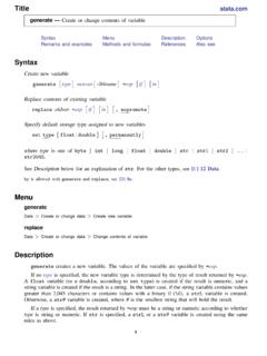
1 Histograms for continuous and categorical variablesSyntaxMenuDescriptionOptions for use in the continuous caseOptions for use in the discrete caseOptions for use in the continuous and discrete casesRemarks and examplesReferencesAlso seeSyntaxhistogramvarname[if] [in] [weight] [,[continuousopts|discreteopts]options]c ontinuousoptsDescriptionMainbin(#)set number of bins to#width(#)set width of bins to#start(#)set lower limit of first bin to#discreteoptsDescriptionMaindiscretesp ecify that data are discretewidth(#)set width of bins to#start(#)set theoretical minimum value to#12 histogram Histograms for continuous and categorical variablesoptionsDescriptionMaindensitydr aw as density.

2 The defaultfractiondraw as fractionsfrequencydraw as frequenciespercentdraw as percentagesbaroptionsrendition of barsaddlabelsadd height labels to barsaddlabopts(markerlabeloptions)affect rendition of labelsDensity plotsnormaladd a normal density to the graphnormopts(lineoptions)affect rendition of normal densitykdensityadd a kernel density estimate to the graphkdenopts(kdensityoptions)affect rendition of kernel densityAdd plotsaddplot(plot)add other plots to the histogramY axis, X axis, Titles, Legend, Overall, Bytwowayoptionsany options documented in [G-3]twowayoptionsfweights are allowed; see[U] >HistogramDescriptionhistogramdraws histograms ofvarname, which is assumed to be the name of a continuousvariable unless thediscreteoption is for use in the continuous case Main bin(#)andwidth(#)are alternatives.

3 They specify how the data are to be aggregated into bins:bin()by specifying the number of bins (from which the width can be derived) andwidth()byspecifying the bin width (from which the number of bins can be derived).If neither option is specified, results are the same as ifbin(k)had been specified, wherek= min{sqrt(N),10 ln(N)/ln(10)}and whereNis the (weighted) number of (#)specifies the theoretical minimum ofvarname. The default isstart(m), wheremis theobserved minimum value Histograms for continuous and categorical variables 3 Specifystart()when you are concerned about sparse data, for instance, if you know thatvarnamecan have a value of 0, but you are concerned that 0 may not be (#), if specified, must be less than or equal tom, or else an error will be for use in the discrete case Main discretespecifies thatvarnameis discrete and that you want each unique value ofvarnameto haveits own bin (bar of histogram).

4 Width(#)is rarely specified in the discrete case; it specifies the width of the bins. The default iswidth(d), wheredis the observed minimum difference between the unique values ()if you are concerned that your data are sparse. For example, in theoryvarnamecould take on the values, say, 1, 2, 3,.., 9, but because of the sparseness, perhaps only thevalues 2, 4, 7, and 8 are observed. Here the default width calculation would producewidth(2),and you would want to specifywidth(1).start(#)is also rarely specified in the discrete case; it specifies the theoretical minimum value ofvarname.

5 The default isstart(m), wheremis the observed minimum withwidth(), specifystart(#)if you are concerned that your data are sparse. In the previousexample, you might also want to specifystart(1).start()does nothing more than add whitespace to the left side of the value of#instart()must be less than or equal tom, or an error will be for use in the continuous and discrete cases Main density,fraction,frequency, andpercentspecify whether you want the histogram scaled todensity units, fractional units, frequencies, or the the height of the bars so that the sum of their areas equals the height of the bars so that the sum of their heights equals the height of the bars so that each bar s height is equal to the numberof observations in the category.

6 Thus the sum of the heights is equal to the total number the height of the bars so that the sum of their heights equals any of the options allowed bygraph twoway bar; see [G-2] graph twoway of the most usefulbaroptionsisbarwidth(#), which specifies the width of the bars invarnameunits. By default,histogramdraws the bars so that adjacent bars just touch. If you wantgaps between the bars, do not specifyhistogram swidth()option which would change howthe histogram is calculated but specify thebaroptionbarwidth()or thehistogramoptiongap, both of which affect only how the bar is be used with that the top of each bar be labeled with the density, fraction, or frequency, asdetermined by thedensity,fraction, histogram Histograms for continuous and categorical variablesaddlabopts(markerlabeloptions)s pecifies how to render the labels atop the bars.

7 See[G-3]markerlabeloptions. Do not specify themarkerlabeloptionmlabel(varname), whichspecifies the variable to be used; this is specified for you ()will accept more options than those documented in [G-3] options allowed bytwoway scatterare also allowed byaddlabopts(); see [G-2]graphtwoway scatter. One particularly useful option isyvarformat(); see [G-3]advancedoptions. Density plots normalspecifies that the histogram be overlaid with an appropriately scaled normal density. Thenormal will have the same mean and standard deviation as the (lineoptions)specifies details about the rendition of the normal curve, such as the colorand style of line used.

8 See [G-2] graph twoway that the histogram be overlaid with an appropriately scaled kernel density estimateof the density. By default, the estimate will be produced using the Epanechnikov kernel with an optimal half-width. This default corresponds to the default ofkdensity; see [R]kdensity. Howthe estimate is produced can be controlled using thekdenopts()option described (kdensityoptions)specifies details about how the kernel density estimate is to be producedalong with details about the rendition of the resulting curve, such as the color and style of lineused.

9 The kernel density estimate is described in [G-2] graph twoway kdensity. As an example,if you wanted to produce kernel density estimates by using the Gaussian kernel with optimalhalf-width, you would specifykdenopts(gauss)and if you also wanted a half-width of 5, youwould specifykdenopts(gauss width(5)). Add plots addplot(plot)allows adding moregraph twowayplots to the graph ; see [G-3]addplotoption. Y axis, X axis, Titles, Legend, Overall, By twowayoptionsare any of the options documented in [G-3]twowayoptions. This includes, mostimportantly, options for titling the graph (see [G-3]titleoptions), options for saving the graph todisk (see [G-3]savingoption), and theby()option, which will allow you to simultaneously graphhistograms for different subsets of the data (see [G-3]byoption).

10 Remarks and are presented under the following headings:Histograms of continuous variablesOverlaying normal and kernel density estimatesHistograms of discrete variablesUse with by()Video exampleFor an example of editing a histogram with the graph Editor, see Pollock (2011, 29 31).histogram Histograms for continuous and categorical variables 5 Histograms of continuous variableshistogramassumes that the variable is continuous, so you need type onlyhistogramfollowedby the variable name:. use (S&P 500). histogram volume(bin=15, start=4103, width= ) 04 Density5,00010,00015,00020,00025,000 Volume (thousands)The small values reported for density on theyaxis are correct; if you added up the area of the bars,you would get 1.