The Fast Fourier Transform (FFT) and MATLAB Examples

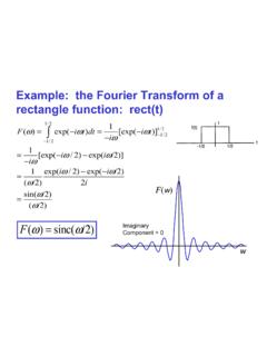
1 The Fast Fourier Transform (FFT)and MATLAB ExamplesLearning ObjectivesDiscrete Fourier transforms (DFTs) and their relationshipto the Fourier transformsImplementation issues with the DFT via the FFTsampling issues (Nyquist criterion)resolution in the frequency domain (zero padding)neglect of negative frequency componentsVf()=vt()exp 2 ift()dt + vt()=Vf()exp 2 ift()df + These Fourier integral pairs normally are performednumerically by sampling the time and frequencydomain functions at discrete values of time andfrequency and then using the discrete Fourier transforms to relate the sampled valuesFast Fourier TransformDiscrete Fourier TransformVpfn()=TNvptj()exp 2 ijn/N()j=0N 1 vptk()=1 TVpfn()exp 2 ikn/N()n=0N 1 T=N time window sampled with Npoints sampling time intervaljtjt= /nfnfnNt= = As with the Fourier transforms, there are different choicesmade for the Discrete Fourier Transform pairs.

2 In general, wecould write:()()()()( ) ()110120exp2/exp2/NpnpjjNpkp nnVfnvtijnNvt n Vfikn N = == = mas long as 121nnN=The indexing could also go from1 to Ninstead of 0 to N-1 Fast Fourier TransformVpfn()=TNvptj()exp 2 ijn/N()j=0N 1 vptk()=1 TVpfn()exp 2 ikn/N()n=0N 1 These discrete Fourier Transforms can be implemented rapidly with the Fast Fourier Transform (FFT) algorithm Fast Fourier TransformFFTs are most efficient if the number of samples, N, isa power of 2. Some FFT software implementations ,57616,769,0254,0965,1201,046,5291,0241, 02465,025256(N/2)log2N(N-1)2 NMathematicaFourier[{a1,a2,..,aN}]1 Narexp 2 ir 1()s 1()/N[]r=1N InverseFourier[{b1,b2,..,bN}]1 Nbsexp 2 ir 1()s 1()/N[]s=1N listsMapleFFT(N, xre, xim)N= 2nxj()exp 2 ijk/N[]j=0N 1 1 NXk()exp 2 ijk/N[]k=0N 1 iFFT(N,Xre,Xim) MATLAB arraysxj()exp 2 ij 1()k 1()/N[]j=1N fft(x)ifft(X)1 NXj()exp 2 ij 1()k 1()/N[]j=1N arraysFast Fourier TransformFFT functionFast Fourier Transformfunction y = FourierT(x, dt)% FourierT(x,dt) computes forward FFT of x with sampling time interval dt% FourierT approximates the Fourier Transform where the integrand of the% Transform is x*exp(2*pi*i*f*t)% For NDE applications the frequency components are normally in MHz, % dt in microseconds [nr, nc] = size(x);if nr == 1N = nc;else N = nr;endy = N*dt*ifft(x).

3 Inverse FFT functionFast Fourier Transformfunction y = IFourierT(x, dt)% IFourierT(x,dt) computes the inverse FFT of x, for a sampling time interval dt% IFourierT assumes the integrand of the inverse Transform is given by% x*exp(-2*pi*i*f*t) % The first half of the sampled values of x are the spectral components for% positive frequencies ranging from 0 to the Nyquist frequency 1/(2*dt)% The second half of the sampled values are the spectral components for% the corresponding negative frequencies. If these negative frequency% values are set equal to zero then to recover the inverse FFT of x we must% replace x(1) by x(1)/2 and then compute 2*real(IFourierT(x,dt))[nr,nc] = size(x);if nr == 1N = nc;elseN = nr;endy =(1/(N*dt))*fft(x);vpt() vt()Vpf() Vf()ifNyquistcriterionT-Ttmaxfs-fsfmaxvp (t)| Vp(f) |tmax T=N tfs 1 t 2fmaxN samplesN samplesFast Fourier Transformvpand Vpin the discrete Fourier transforms are periodic do we guarantee these represent non-periodic pulses?

4 The use of linspace and s_space functions for FFTsand inverse FFTsT = =In the example above N = 8, T= so 1/ 8 = =>> t = linspace(0,1, 8);>> dt = t(2) -t(1)dt = get the proper sampled values and the correct t we can use the alternate function s_space (it s on the ftp site)>> t = s_space(0,1, 8);>> dt = t(2)-t(1)dt = >> t = linspace(0,1, 512);>> dt = t(2) - t(1)dt = >> t = s_space(0,1, 512);>> dt = t(2) - t(1)dt = you are using many points the difference is not large if we use either linspace or s_space but the difference is still there>> format long>> t = linspace(0, 1, 500);>> dt = t(2) -t(1)dt = >> t = s_space(0, 1, 500);>> dt = t(2) -t(1)dt = (t)N samples2Tv(t)2N samplesfs= 1/ t| V (f) |N samples f f =1/T tfs= 1/ t| V (f) |2N samples t f =1/2T fzero padding Fast Fourier Transform >> t =s_space(0, 4, 16);>> v = t.

5 *(t < ) + (1-t).*(t >= >> h = plot(t, v, 'ko');>> set(h, 'MarkerFaceColor', 'k')>> axis([ 0 4 0 ])>> dt = t(2) - t(1)dt = padding example>> f =s_space(0, 1/dt, 16);>> vf = FourierT(v, dt);>> h = plot(f, abs(vf), 'ko');>>axis([ 0 4 0 ])>> set(h, 'MarkerFaceColor', 'k')>> df = f(2) - f(1)df = >> vt2 =[v, zeros(1,16)];>> vf2 = FourierT(vt2, dt);>> h = plot(f, abs(vf2), 'ko');??? Error using ==> plotVectors must be the same lengths.>> f =s_space(0, 1/dt, 32);>> h = plot(f, abs(vf2), 'ko');>> set(h, 'MarkerFaceColor', 'k')>>axis([ 0 4 0 ])could also use vt2 = padarray(v,[0, 16], 0, post );>> df=f(2) - f(1)df = the former dfsame sampling frequencyNow, pad the original signal with >> t =s_space(0, 4, 512);>> v = t.*(t < ) + (1-t).)

6 *(t >= >> dt = t(2) -t(1)dt = >> fs =1/dtfs = 128>> f =s_space(0, fs, 512);>> vf =FourierT(v, dt);>> plot(f, abs(vf))Now, use a much higher sampling >> h = plot(f(1:20), abs(vf(1:20)), 'ko');>> set(h, 'MarkerFaceColor', 'k')To see the frequency spectrum on a finer : we had some aliasing before>> vt =IFourierT(vf, dt);>> plot(t, real(vt))If we do the inverse FFT we do again recover the time can do multiple FFTs or IFFT sall at once if we place the data in columns>> t =s_space(0, 4, 16);>> v = t.*(t < ) + (1-t).*(t >= >> dt = t(2) - t(1);>> mv= [ v' v' v'];>> mvf = FourierT(mv, dt);>> vf1 = mvf(:,1);>> f = s_space(0, 1/dt, 16);>> h = plot(f, abs(vf1)', 'ko')>> set(h, 'MarkerFaceColor', 'k') that even though there is aliasing here if we do the inverse FFT of these samples we do recover the original time samples:>> v1 =IFourierT(vf1,dt);>> h=plot(t, real(v1), 'ko');>> set(h, 'MarkerFaceColor', 'k') Fourier TransformFFT Examples using the function:function y = pulse_ref(A,F,N, t)y = A*(1 -cos(2*pi*F* )).))

7 *cos(2*pi*F*t).*(t >= 0 & t <= N/F);()()()()1cos2 /cos20/0 AFt NFttN Fytotherwise << = A .. controls the amplitudeF .. controls the dominant frequency in the pulseN .. controls the number of cycles (amount of "ringing")in the pulse and hence the bandwidthMATLAB function:>> t = s_space(0,5,512);>> dt = t(2)- t(1)dt = >> y=pulse_ref(1,5,3,t);>> plot(t, y)>> yf1=FourierT(y,dt);>> f=s_space(0, 1/dt, 512);>> f(end)ans = >> plot(f, abs(yf1))Frequency spectrum for relatively wideband pulseif t is in secf is in MHzsampling frequencyNyquist frequency= sampling >> plot(f(1:100), abs(yf1(1:100)))Expanded view0 20 >> y = pulse_ref(1,5,5,t);>> yf2 = FourierT(y, dt);>> plot(f(1:100), abs(yf2(1:100)))Somewhat morenarrow band pulse(only 0 - 20 MHzshown) >> y = pulse_ref(1,5,10,t);>> yf3 = FourierT(y, dt).

8 >> plot(f(1:100), abs(yf3(1:100)))Decrease bandwidtheven more(only 0 - 20 MHzshown) f is not quite adequate here f =1/T = 1/5 MHz>> plot(f(1:50), abs(yf3(1:50)))Show plot in more can improve these results with zero padding of our signalzero paddingnow, have 1024 points over 10microseconds, so dt is same butT = Ndt is twice as large012345678910-2-1012>> t=s_space(0, 10, 1024);>> y=pulse_ref(1, 5,10, t);>> plot(t,y)>> dt = t(2) -t(1)dt = , originally, we hadt = s_space(0,5, 512);we could also zero pad viat = [t, zeros(1, 512)];>> yf4 = FourierT(y, dt);>> f = s_space(0, 1/dt, 1024);>> plot(f(1:100), abs(yf4(1:100)))Improved representation of thespectrum f = 1/T = 1/10 >> y = IFourierT(yf3, dt);>> plot(t , real(y));Example inverse FFT (of yf3)real part is taken here to eliminate any smallimaginary components due to numerical round | Vp(f) |N samplespositive frequencycomponentsnegative frequencycomponentsfsfmax| Vp(f) |N samplespositive frequencycomponents?

9 In time domainV f()=V*f()if v(t) is realFast Fourier Transformvt()=Vf()exp 2 ift()df + vt()2 i2 Hvt()[]=Vf()0+ exp 2 ift()dfHilbert Transform of v(t)sovt()=2 ReVf()0+ exp 2 ift()df Fast Fourier Transform >> t = s_space(0,5, 512);>> y = pulse_ref(1,5,10,t);>> plot(t, y)>> yf= FourierT(y, dt);>> yf5 = yf .*(f < 50);>> plot(f, abs(yf5))zero negativefrequency componentsThrowing out negative frequency componentsnow, do the inverse FFTon just these positivefrequency >> yf5(1) = yf5(1)/2;>> y = 2*real(IFourierT(yf5, dt));>> plot(t, y)when throwing out negative frequencycomponents, need to divide dc value by half also (not needed if dc value is zero oralready very small)012345-2-1012 ReferencesWalker, , Fast Fourier Transforms, CRC Press, 1996 Burrus, and Parks, DFT/FFT and Convolution Algorithms, John Wiley and Sons, New York, Fourier Transform