Transcription of The Gaussian distribution - Washington University in St. Louis
1 4 3 2 = 0, = 1 = 1, =1/2 = 0, = 2 Figure 1: Examples of univariate GaussianpdfsN(x; , 2).The Gaussian distributionProbably the most-important distribution in all of statistics is theGaussian distribution ,also calledthenormal Gaussian distribution arises in many contexts and is widely used formodeling continuous random probability density function of the univariate (one-dimensional) Gaussian distribution isp(x| , 2) =N(x; , 2) =1 Zexp( (x )22 2).The normalization constantZisZ= 2 parameters and 2specify the mean and variance of the distribution , respectively: =E[x]; 2= var[x].Figure 1 plots the probability density function for several sets of parameters( , 2).
2 The distributionis symmetric around the mean and most of the density ( ) is contained within 3 of may extend the univariate Gaussian distribution to a distribution overd-dimensional vectors,producing a multivariate analog. The probablity density function of the multivariate Gaussiandistribution isp(x| , ) =N(x; , ) =1 Zexp( 12(x )> 1(x )).The normalization constantZisZ= det(2 ) = (2 )d/2(det )1 4 2024 4 2024x1x2(a) =[1 00 1] 4 2024 4 2024x1x2(b) =[11/21/21] 4 2024 4 2024x1x2(c) =[1 1 13]Figure 2: Contour plots for example bivariate Gaussian distributions. Here =0for all these equations, we can see that the multivariate density coincides with the univariatedensity in the special case when is the scalar , the vector speci es the mean of the multivariate Gaussian distribution .
3 The matrix speci es thecovariancebetween each pair of variables inx: = cov(x,x) =E[(x )(x )>].Covariance matrices are necessarily symmetric andpositive semide nite,which means their eigen-values are nonnegative. Note that the density function above requires that bepositive de nite,orhave strictly positive eigenvalues. A zero eigenvalue would result in a determinant of zero, makingthe normalization dependence of the multivariate Gaussian density onxis entirely through the value of thequadratic form 2= (x )> 1(x ).The value (obtained via a square root) is called theMahalanobis distance,and can be seen as ageneralization of theZscore(x ) , often encountered in understand the behavior of the density geometrically, we can set the Mahalanobis distance to aconstant.
4 The set of points inRdsatisfying =cfor any given valuec >0is an ellipsoid withthe eigenvectors of de ning the directions of the principal 2 shows contour plots of the density of three bivariate (two-dimensional) Gaussian distribu-tions. The elliptical shape of the contours is Gaussian distribution has a number of convenient analytic properties, some of which wedescribe we will have a set of variablesxwith a joint multivariate Gaussian distribution , but only beinterested in reasoning about a subset of these variables. Supposexhas a multivariate Gaussiandistribution:p(x| , ) =N(x, , ).2 4 2024 4 2024x1x2(a)p(x| , ) 4 (x1)(b)p(x1| 1, 11) =N(x1; 0,1)Figure 3: Marginalization example.
5 (a) shows the joint density overx= [x1,x2]>; this is the samedensity as in Figure 2(c). (b) shows the marginal density us partition the vector into two components:x=[x1x2].We partition the mean vector and covariance matrix in the same way: =[ 1 2] =[ 11 12 21 22].Now the marginal distribution of the subvectorx1has a simple form:p(x1| , ) =N(x1, 1, 11),so we simply pick out the entries of and corresponding 3 illustrates the marginal distribution ofx1for the joint distribution shown in Figure 2(c).ConditioningAnother common scenario will be when we have a set of variablesxwith a joint multivariateGaussian prior distribution , and are then told the value of a subset of these variables.
6 We maythen condition our prior distribution on this observation, giving a posterior distribution over theremaining again thatxhas a multivariate Gaussian distribution :p(x| , ) =N(x, , ),and that we have partitioned as before:x= [x1,x2]>. Suppose now that we learn the exact valueof the subvectorx2. Remarkably, the posterior distributionp(x1|x2, , )3 4 2024 4 2024x1x2(a)p(x| , ) 4 (x1|x2= 2)p(x1)(b)p(x1|x2, , ) =N(x1; 2/3,(2/3)2)Figure 4: Conditioning example. (a) shows the joint density overx= [x1,x2]>, along with theobservation valuex2= 2; this is the same density as in Figure 2(c). (b) shows the conditionaldensity ofx1givenx2= a Gaussian distribution !
7 The formula isp(x1|x2, , ) =N(x1; 1|2, 11|2),with 1|2= 1+ 12 122(x2 2); 11|2= 11 12 122 we adjust the mean by an amount dependent on: (1) the covariance betweenx1andx2, 12,(2) the prior uncertainty inx2, 22, and (3) the deviation of the observation from the prior mean,(x2 2). Similarly, we reduce the uncertainty inx1, 11, by an amount dependent on (1) and (2).Notably, the reduction of the covariance matrix doesnotdepend on the values we that ifx1andx2are independent, then 12=0, and the conditioning operation does notchange the distribution ofx1, as 4 illustrates the conditional distribution ofx1for the joint distribution shown in Figure 2(c),after observingx2= multiplicationAnother remarkable fact about multivariate Gaussian density functions is that pointwise multipli-cation gives another (unnormalized) Gaussianpdf:N(x; , )N(x; ,P) =1ZN(x; ,T),whereT= ( 1+P 1) 1 =T( 1 +P 1 )Z 1=N( ; , +P) =N( ; , +P).
8 4 4 2024 4 2024x1x2(a)p(x| , ) 4 2024 4 2024x1x2(b)p(y| , ,A,b)Figure 5: A ne transformation example. (a) shows the joint density overx= [x1,x2]>; this is thesame density as in Figure 2(c). (b) shows the density ofy=Ax+b. The values ofAandbaregiven in the text. The density of the transformed vector is another probability density functions are closed under convolutions. Letxandybed-dimensionalvectors, with distributionsp(x| , ) =N(x; , );p(y| ,P) =N(y; ,P).Then the convolution of their density functions is another Gaussianpdf:f(y) = N(y x; ,P)N(x; , ) dx=N(y; + , +P),where the mean and covariances add in the we assume thatxandyare independent, then the distribution of their sumz=x+ywillalso have a multivariate Gaussian distribution , whose density will precisely the convolution of theindividual densities:p(z| , , ,P) =N(z; + , +P).
9 These results will often come in ne transformationsConsider ad-dimensional vectorxwith a multivariate Gaussian distribution :p(x| , ) =N(x, , ).Suppose we wish to reason about an a ne transformation ofxintoRD,y=Ax+b, whereA RD dandb RD. Thenyhas aD-dimensional Gaussian distribution :p(y| , ,A,b) =N(y,A +b,A A>).5 Figure 5 illustrates an a ne transformation of the vectorxwith the joint distribution shown inFigure 2(c), for the valuesA=[1/5 3/51/23/10];b=[1 1].The density has been rotated and translated, but remains a parametersThed-dimensional multivariate Gaussian distribution is speci ed by the parameters and .Without any further restrictions, specifying requiresdparameters and specifying requires afurther(d2)=d(d 1)2.
10 The number of parameters therefore grows quadratically in the dimension,which can sometimes cause di culty. For this reason, we sometimes restrict the covariance matrix in some way to reduce the number of choices are to set = diag , where is a vector of marginal variances, and = 2I, aconstant diagonal matrix. Both of these options assume independence between the variables former case is more exible, allowing a di erent scale parameter for each entry, whereas thelatter assumes an equal marginal variance of 2for each variable. Geometrically, the densities areaxis-aligned, as in Figure 2(a), and in the latter case, the isoprobability contours are spherical (alsoas in Figure 2(a)).