Transcription of The GLM Procedure
1 Chapter 30 The GLM ProcedureChapter Table of ..1468 GETTING ..1469 PROC GLM for Quadratic Least Squares Regression ..1479 ABSORBS tatement .. Statement ..1483 ESTIMATE Statement ..1486 FREQS tatement ..1487 IDStatement ..1493 MEANSS tatement ..1497 MODELS tatement ..1504 OUTPUTS tatement ..1507 RANDOM Statement ..1510 REPEATED Statement ..1511 TEST .. Testing in PROC GLM ..1526 Absorption ..1532 Specification of ESTIMATE Expressions ..1536 Comparing Chapter 30. The GLM ProcedureMeansVersusLS-Means ..1538 Multiple Comparisons ..1558 Repeated Measures Analysis of Effects Analysis ..1567 MissingValues ..1574 OutputDataSets ..1574 DisplayedOutput ..1576 ODST ableNames .. Balanced Data from Randomized Complete Block with MeansComparisonsandContrasts ..1580 Example Regression with Mileage Data ..1586 Example Unbalanced ANOVA for Two-Way Design with Interaction .. Repeated Measures Analysis of Variance ..1609 Example Mixed Model Analysis of Variance Using the Analyzing a Doubly-multivariate Repeated Measures Design.
2 OnlineDoc : Version 8 Chapter 30 The GLM ProcedureOverviewThe GLM Procedure uses the method of least squares to fit general linear the statistical methods available in PROC GLM are regression, analysis ofvariance, analysis of covariance, multivariate analysis of variance, and partial GLM analyzes data within the framework of General linear models. PROCGLM handles models relating one or several continuous dependent variables to one orseveral independent variables. The independent variables may be eitherclassificationvariables, which divide the observations into discrete groups, , the GLM Procedure can be used for many different analyses, including simple regression multiple regression analysis of variance (ANOVA), especially for unbalanced data analysis of covariance response-surface models weighted regression polynomial regression partial correlation multivariate analysis of variance (MANOVA) repeated measures analysis of variancePROC GLM FeaturesThe following list summarizes the features in PROC GLM: PROC GLM enables you to specify any degree of interaction (crossed effects)and nested effects.
3 It also provides for polynomial, continuous-by- class , andcontinuous-nesting- class effects. Through the concept of estimability, the GLM Procedure can provide tests ofhypotheses for the effects of a linear model regardless of the number of missingcells or the extent of confounding. PROC GLM displays the Sum of Squares(SS) associated with each hypothesis tested and, upon request, the form of theestimable functions employed in the test. PROC GLM can produce the generalform of all estimable Chapter 30. The GLM Procedure The REPEATED statement enables you to specify effects in the model thatrepresent repeated measurements on the same experimental unit for the sameresponse, providing both univariate and multivariate tests of hypotheses. The RANDOM statement enables you to specify random effects in the model;expected mean squares are produced for each Type I, Type II, Type III, TypeIV, and contrast mean square used in the analysis. Upon request,Ftests usingappropriate mean squares or linear combinations of mean squares as error termsare performed.
4 The ESTIMATE statement enables you to specify anLvector for estimating alinear function of the parametersL . The CONTRAST statement enables you to specify a contrast vector or matrixfor testing the hypothesis thatL =0. When specified, the contrasts are alsoincorporated into analyses using the MANOVA and REPEATED statements. The MANOVA statement enables you to specify both the hypothesis effectsand the error effect to use for a multivariate analysis of variance. PROC GLM can create an output data set containing the input dataset in addi-tion to predicted values, residuals, and other diagnostic measures. PROC GLM can be used interactively. After specifying and running a model,a variety of statements can be executed without recomputing the model param-eters or sums of squares. For analysis involving multiple dependent variables but not the MANOVAor REPEATED statements, a missing value in one dependent variable doesnot eliminate the observation from the analysis for other dependent GLM automatically groups together those variables that have the samepattern of missing values within the data set or within a BY group.
5 This en-sures that the analysis for each dependent variable brings into use all GLM Contrasted with Other SAS ProceduresAs described previously, PROC GLM can be used for many different analyses andhas many special features not available in other SAS procedures. However, for sometypes of analyses, other procedures are available. As discussed in the PROC GLMfor Unbalanced ANOVA and PROC GLM for Quadratic Least Squares Regression sections (beginning on page 1469), sometimes these other procedures are more effi-cient than PROC GLM. The following procedures perform some of the same analysesas PROC GLM:ANOVA performs analysis of variance for balanced designs. The ANOVA Procedure is generally more efficient than PROC GLM for mixed linear models by incorporating covariance structures inthe model fitting process. Its RANDOM and REPEATED state-ments are similar to those in PROC GLM but offer different OnlineDoc : Version 8 PROC GLM for Unbalanced ANOVA 1469 NESTED performs analysis of variance and estimates variance componentsfor nested random models.
6 The NESTED Procedure is generallymore efficient than PROC GLM for these nonparametric one-way analysis of rank scores. This canalso be done using the RANK Procedure and PROC simple linear regression. The REG Procedure allows sev-eral MODEL statements and gives additional regression diagnos-tics, especially for detection of collinearity. PROC REG also cre-ates plots of model summary statistics and regression quadratic response-surface regression, and canonical andridge analysis. The RSREG Procedure is generally recommendedfor data from a response surface the means of two groups of observations. Also, tests forequality of variances for the two groups are available. The TTEST Procedure is usually more efficient than PROC GLM for this typeof variance components for a general linear StartedPROC GLM for Unbalanced ANOVAA nalysis of variance, or ANOVA, typically refers to partitioning the variation in avariable s values into variation between and within several groups or classes of ob-servations.
7 The GLM Procedure can perform simple or complicated ANOVA forbalanced or unbalanced example discusses a2 2 ANOVA model. The experimental design is a fullfactorial, in which each level of one treatment factor occurs at each level of the othertreatment factor. The data are shown in a table and then read into a SAS data Analysis of Unbalanced 2-by-2 Factorial ;data exp;input A $ B $ Y @@;datalines;A1 B1 12 A1 B1 14 A1 B2 11 A1 B2 9A2 B1 20 A2 B1 18 A2 B2 17;SAS OnlineDoc : Version 81470 Chapter 30. The GLM ProcedureNote that there is only one value for the cell withA= A2 andB= B2 . Since onecell contains a different number of values from the other cells in the table, this is anunbalanced following PROC GLM invocation produces the glm; class A B;model Y=A B A*B;run;Both treatments are listed in the class statement because they are *Bdenotes the interaction of theAeffect and theBeffect. The resultsare shown in Figure and Figure of Unbalanced 2-by-2 FactorialThe GLM ProcedureClass Level InformationClass Levels ValuesA 2 A1 A2B 2 B1 B2 Number of observations 7 Figure Level InformationFigure displays information about the classes as well as the number of observa-tions in the data set.
8 Figure shows the ANOVA table, simple statistics, and testsof OnlineDoc : Version 8 PROC GLM for Quadratic Least Squares Regression 1471 Analysis of Unbalanced 2-by-2 FactorialThe GLM ProcedureDependent Variable: YSum ofSource DF Squares Mean Square F Value Pr > FModel 3 3 Total 6 Coeff Var Root MSE Y DF Type I SS Mean Square F Value Pr > FA 1 1 *B 1 DF Type III SS Mean Square F Value Pr > FA 1 1 *B 1 Table and Tests of EffectsThe degrees of freedom may be used to check your data.
9 The Model degrees offreedom for a2 2factorial design with interaction are(ab 1),whereais thenumber of levels ofAandbis the number of levels ofB; in this case,(2 2 1)=3. The Corrected Total degrees of freedom are always one less than the number ofobservations used in the analysis; in this case,7 1= overallFtest is significant(F=15:29;p=0:0253), indicating strong evidencethat the means for the four differentA Bcells are different. You can further analyzethis difference by examining the individual tests for each types of estimable functions of parameters are available for testing hypothesesin PROC GLM. For data with no missing cells, the Type III and Type IV estimablefunctions are the same and test the same hypotheses that would be tested if the datawere balanced. Type I and Type III sums of squares are typically not equal whenthe data are unbalanced; Type III sums of squares are preferred in testing effects inunbalanced cases because they test a function of the underlying parameters that isindependent of the number of observations per treatment to a significance level of5%( =0:05),theA*Binteraction is not signif-icant(F=0:20;p=0:6850).
10 This indicates that the effect ofAdoes not depend onthe level ofBand vice versa. Therefore, the tests for the individual effects are valid,showing a significantAeffect(F=33:80;p=0:0101)but no significantBeffect(F=5:00;p=0:1114).SAS OnlineDoc : Version 81472 Chapter 30. The GLM ProcedurePROC GLM for Quadratic Least Squares RegressionIn polynomial regression, the values of a dependent variable (also called a responsevariable) are described or predicted in terms of polynomial terms involving one ormore independent or explanatory variables. An example of quadratic regression inPROC GLM follows. These data are taken from Draper and Smith (1966, p. 57).Thirteen specimens of 90/10 Cu-Ni alloys are tested in a corrosion-wheel setup inorder to examine corrosion. Each specimen has a certain iron content. The wheel isrotated in salt sea water at 30 ft/sec for 60 days. Weight loss is used to quantify thecorrosion. Thefevariable represents the iron content, and thelossvariable denotesthe weight loss in milligrams/square decimeter/day in the following DATA Regression in PROC GLM ;data iron;input fe loss @ ;The GPLOT Procedure is used to request a scatter plot of the response variable versusthe independent c=blue;proc gplot;plot loss*fe / vm=1;run;The plot in Figure displays a strong negative relationship between iron contentand corrosion resistance, but it is not clear whether there is curvature in this OnlineDoc : Version 8 PROC GLM for Quadratic Least Squares Regression 1473 Figure following statements fit a quadratic regression model to the data.