Transcription of The OC Curve of Attribute Acceptance Plans
1 Copyright 2009 by Ombu Enterprises, LLC The OC Curve of Attribute Acceptance Plans Page 1 of 7 The OC Curve of Attribute Acceptance Plans The Operating Characteristic (OC) Curve describes the probability of accepting a lot as a function of the lot s quality. Figure 1 shows a typical OC Curve . Operating Characteristic nonconforming, pProbability of Acceptance , Pa Figure 1 Typical Operating Characteristic (OC) Curve The Shape of the OC Curve The first thing to notice about the OC Curve in Figure 1 is the shape; the Curve is not a straight line. Notice the roughly S shape. As the lot percent nonconforming increases, the probability of Acceptance decreases, just as you would expect. Historically, Acceptance sampling is part of the process between a part s producer and consumer.
2 To help determine the quality of a process (or lot) the producer or consumer can take a sample instead of inspecting the full lot. Sampling reduces costs, because one needs to inspect or test fewer items than looking at the whole lot. Sampling is based on the idea that the lots come from a process that has a certain nonconformance rate (but there is another view described below). The concept is that the consumer will accept all the producer s lots as long as the process percent nonconforming is below a prescribed level. This produces the, so called, ideal OC Curve shown in Figure 2. When the process percent nonconforming is below the prescribed level, in this example, the probability of Acceptance is 100%. For quality worse than this level, higher than 4%, the probability of Acceptance immediately drops to 0%.
3 The dividing line between 100% and 0% Acceptance is called the Acceptable Quality Level (AQL). Copyright 2009 by Ombu Enterprises, LLC The OC Curve of Attribute Acceptance Plans Page 2 of 7 The original idea for sampling takes a simple random sample, of n units, from the lot. If the number of nonconforming items is below a prescribed number, called the Acceptance number and denoted c, we accept the lot. If the sample contains more nonconforming items, we reject the lot. Operating Characteristic nonconforming, pProbability of Acceptance , Pa Figure 2 Ideal OC Curve The only way to realize the ideal OC Curve is 100% inspection. With sampling, we can come close. In general, as the sample size increases, keeping the Acceptance number proportional, the OC Curve approaches the ideal, as shown in Figure 3.
4 Similarly, as the Acceptance number, c, gets larger for a given sample size, n, the OC Curve approaches the ideal. Figure 4 illustrates the relationship. Some Specific Points on the OC Curve Because sampling doesn t allow the ideal OC Curve , we need to consider certain risks. The first risk is that the consumer will reject a lot that satisfies the established conditions, , the process quality is acceptable, but, by the luck of the draw, there are too many nonconforming items in the sample. This is called the producer s risk, and is denoted by the Greek letter . The second risk is that the consumer will accept a lot that doesn t meet the conditions, , by the luck of the draw there are not many nonconforming items in the sample, so the lot is accepted.
5 This is the consumer s risk and is denoted by the Greek letter . The literature contains a variety of typical values for and , but common values are 5% and 10%. When we locate these values on the OC Curve , expressed in terms of probability of Acceptance , we actually locate 1 . Copyright 2009 by Ombu Enterprises, LLC The OC Curve of Attribute Acceptance Plans Page 3 of 7 Operating Characteristic nonconforming, pProbability of Acceptance , Pan=200, c=4n=100, c=2n= 50, c=1 Figure 3 As n Increases the OC Curve Approaches the Ideal Operating Characteristic nonconforming, pProbability of Acceptance , Pan=100, c=2n=100, c=1n=100, c=0 Figure 4 As c Increases, for Fixed n, the OC Curve Approaches the Ideal Copyright 2009 by Ombu Enterprises, LLC The OC Curve of Attribute Acceptance Plans Page 4 of 7 These points correspond to specific values of lot quality and they have a variety of names.
6 The point associated with 1 is often called the Acceptable Quality Limit or AQL. This is not necessarily the same AQL used to describe the ideal OC Curve . For an of 5% this means a process operating at the AQL will have 95% of its lots accepted by the sampling plan . Similarly, the point associated with is often called, in contrast, the Rejectable Quality Limit or RQL. A process operating at the RQL will have 5% of its lots accepted by the sampling plan . Lastly, some authors consider the process quality where the lots have a 50% probability of Acceptance . This is called the Indifference Quality Limit or IQL. Figure 5 illustrates these points. Operating Characteristic nonconforming, pProbability of Acceptance , PaIQLRQLAQL1 - Figure 5 Specific Points on the OC Curve A Stream of Lots and the Binomial Distribution We described the OC Curve in terms of a process that produces a series of lots.
7 This leads us to recognize that the underlying distribution is the binomial. In the binomial distribution, there are two possible outcomes. The items in the sample are either conforming or nonconforming. In addition, the probably of selecting a nonconforming item doesn t change as a result of the sample. Since we are sampling from a process, the potentially infinite number of items is not impacted by taking the sample. When the producer presents lots for Acceptance , they often come from a process that is operating at some quality level, , the process produces a certain percentage of nonconforming items. The probability of obtaining a specified number of nonconforming items, Pr(x), from a sample of n items with percent nonconforming, denoted p, is given by the binomial distribution.
8 Copyright 2009 by Ombu Enterprises, LLC The OC Curve of Attribute Acceptance Plans Page 5 of 7 ()nxppxnxxnx,,1,0,1)Pr(..= = In a single sample plan we accept the lot if the number of nonconforming items is c or less. This means we are interesting in the probability of 0, 1, .., c items. We write this as () = = cixixppincx01)Pr( The probability of accepting the lot is the probability that there are c or fewer nonconforming items in the sample. This is the equation above, and is what we plot as the OC Curve . The Isolated Lot And The Hypergeometric Distribution The binomial distribution applies when we consider lots coming from an ongoing production process. Sometimes we consider isolated lots, or we are interested in a specific lot.
9 In these cases, we need to realize that taking the sample, because we sample without replacement, changes the probability of the next item in the sample. In these cases, we need the hypergeometric distribution. () =nNxndNxdxPr Here, N is the lot size, n is the sample size, and d is the number of nonconforming items in the lot. If we are interested in determining the probability of c or fewer nonconforming items in the sample then we write: () = = cinNindNidcx0Pr We can use this equation to draw the OC Curve for the isolated lot. Often, the risk is applied to each lot, instead of the stream of lots. In these cases, the quality level corresponding to a probability of Acceptance equal to is called the Lot Tolerance Percent Defective (LTPD).
10 Single and Double Sample Plans The material above discusses sampling Plans in which we draw one sample from the lot. This is called a single sample plan . We describe the plan by a set of parameters: n is the sample size, Copyright 2009 by Ombu Enterprises, LLC The OC Curve of Attribute Acceptance Plans Page 6 of 7 c is the maximum number of nonconforming items allowed for Acceptance , and r is the minimum number of nonconforming items allowed for rejection. In a single sample plan r and c differ by 1. In contrast, there are double sampling Plans in which we take the first sample and make one of three decisions: accept, reject, or take a second sample. If we take the second sample, we then make an accept/reject decision. As described above the set of parameters used to describe a double sample plan are: ni is the ith sample size, ci is the maximum number of nonconforming items allowed for Acceptance on the ith sample, and ri is the minimum number of nonconforming items allowed for rejection on the ith sample.