Time Series Forecasting Methods

1 IntroductionUnivariate ForecastingConclusionsTime Series Forecasting MethodsNate DerbyStatis Pro Data AnalyticsSeattle, WA, USAC algary SAS Users Group, 11/12/09 Nate DerbyTime Series Forecasting Methods1 / 43 IntroductionUnivariate ForecastingConclusionsOutline1 IntroductionObjectivesStrategies2 Univariate ForecastingSeasonal Moving AverageExponential SmoothingARIMA3 ConclusionsWhich Method?Are Our Results Better?What s Next?Nate DerbyTime Series Forecasting Methods2 / 43 IntroductionUnivariate ForecastingConclusionsObjectivesStrategi esObjectivesWhat is time Series data?What do we want out of a forecast?Long-term or short-term?Broken down into different categories/ time units?Do we wantprediction intervals?Do we want to measure effect ofXonY? (scenarioforecasting)What Methods are out there to forecast/analyze them?How do we decide which method is best?How can we use SAS for all this?Nate DerbyTime Series Forecasting Methods3 / 43 IntroductionUnivariate ForecastingConclusionsObjectivesStrategi esWhat is time Series Data?

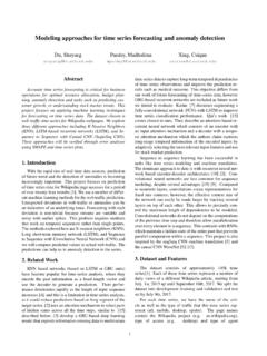
2 time Series data = Data with a pattern ( trend ) over time trend = Get wrong myPROC DerbyTime Series Forecasting Methods4 / 43 IntroductionUnivariate ForecastingConclusionsObjectivesStrategi es ! " " # $ % # & " '( )* + , " ! $ - " ./00/10200210300310400410100110500510600 0/7480/7100/71/0/7120/7130/7140/7110/715 0/7160/7190/7180/7500/75/0/752!"#$"%&'() **&%+&#*',)%-' ./.'0'1&2-' .3456789*)%:*'8;'<)**&%+&#*=Nate DerbyTime Series Forecasting Methods5 / 43 IntroductionUnivariate ForecastingConclusionsObjectivesStrategi esBase Data SetNate DerbyTime Series Forecasting Methods6 / 43 IntroductionUnivariate ForecastingConclusionsObjectivesStrategi esWhat do we want out of a Forecast?Long-term:Involvesmanyassumptio ns! ( , global warming)Involves tons of : In the long run we are all dead .We ll focus on the short categories?Two strategies for Forecasting A, B and C:1 Forecast their combined total, then break it down them : Do (1) unless percentages are DerbyTime Series Forecasting Methods7 / 43 IntroductionUnivariate ForecastingConclusionsObjectivesStrategi esWhat do we want out of a Forecast?

3 Different time units?Two strategies for Forecasting at two different time units ( ,daily and weekly):1 Forecast weekly, then break down into days by daily, then aggregate into : Idea: Do (1) unless percentages are we want prediction intervals?Prediction interval = Interval where data point will be with90/95/99% , we want them!Nate DerbyTime Series Forecasting Methods8 / 43 IntroductionUnivariate ForecastingConclusionsObjectivesStrategi esWhat do we want out of a Forecast?Do we want to measure effect ofXonY?Ex: Marketing campaign calls to call to do, butAllows for scenario Forecasting !Idea: Do it, but only with most Questions: Basis of this talk:What Methods are out there to forecast/analyze them?How do we decide which method is best?How can we use SAS for all this? Methods will DerbyTime Series Forecasting Methods9 / 43 IntroductionUnivariate ForecastingConclusionsObjectivesStrategi esStrategiesTwo stages:Univariate(one variable) Forecasting :ForecastsYfrom trend us a basic (many variables) Forecasting :ForecastsYfrom trend and other variablesX1,X2.

4 Allows for what if scenario or may not make more accurate DerbyTime Series Forecasting Methods10 / 43 IntroductionUnivariate ForecastingConclusionsSeasonal Moving AverageExponential SmoothingARIMAU nivariate Forecasting - IntroGives us a benchmark for comparing multivariate give better forecasts than Methods can be extended to three Methods :Seasonal moving average(verysimple)Exponential smoothing(simple)ARIMA(complex)More complex Methods , for later on (for me):State space(promising)Bayesian(maybe .. )Wavelets?(forget it!)Nate DerbyTime Series Forecasting Methods11 / 43 IntroductionUnivariate ForecastingConclusionsSeasonal Moving AverageExponential SmoothingARIMAOnce Again ..Q: Why not usePROC REG?Yt= 0+ 1Xt+ZtA: We can get misleading results (see myPROC REGpaper).Nate DerbyTime Series Forecasting Methods12 / 43 IntroductionUnivariate ForecastingConclusionsSeasonal Moving AverageExponential SmoothingARIMAS easonal Moving AverageSimple but sometimes effective!

5 Moving Average:Forecast=Average of Moving Average:Forecast=Average of a certain point, forecast the same for each of t allow for a based on amodel No prediction DerbyTime Series Forecasting Methods13 / 43 IntroductionUnivariate ForecastingConclusionsSeasonal Moving AverageExponential SmoothingARIMASAS CodeMaking lags in aDATA step (to make the averages) is not fun:Making 4 lags(Brocklebank and Dickey, p. 45)DATA movingaverage;..RETAIN date pass1-pass4;OUTPUT;pass4=pass3;pass3=pas s2;pass2=pass1;pass1=pass;RUN;Nate DerbyTime Series Forecasting Methods14 / 43 IntroductionUnivariate ForecastingConclusionsSeasonal Moving AverageExponential SmoothingARIMASAS CodeMuch easier with a trick withPROC = averaging over past 5 years on that same month:Yt=15(Yt 12+Yt 24+Yt 36+Yt 48+Yt 60) Forecasting 3 weeks ahead, seasonal moving averagePROC ARIMA data=airline;IDENTIFY var=pass noprint;ESTIMATE p=( 12, 24, 36, 48, 60 ) q=0 ar= noconstant noprint;FORECAST lead=12 out=foremave id=date interval=month noprint;RUN;QUIT;Nate DerbyTime Series Forecasting Methods15 / 43 IntroductionUnivariate ForecastingConclusionsSeasonal Moving AverageExponential SmoothingARIMA !

6 " " # $ % # & " '( )* + , " ! $ - " ./00/10200210300310400410100110500510600 0/7480/7100/71/0/7120/7130/7140/7110/715 0/7160/7190/7180/7500/75/0/752!"#$"%&'() **&%+&#*',)%-' ./.'0'1&2-' .3456789*)%:*'8;'<)**&%+&#*=Nate DerbyTime Series Forecasting Methods16 / 43 IntroductionUnivariate ForecastingConclusionsSeasonal Moving AverageExponential SmoothingARIMA ! " " # $ % # & " '( )* + , " ! $ - " ./00/10200210300310400410100110500510600 0/7480/7100/71/0/7120/7130/7140/7110/715 0/7160/7190/7180/7500/75/0/752!"#$"%&'() **&%+&#*',)%-' ./.'0'1&2-' .345 67"%+'!7&#)+&'86#&2)*9*Nate DerbyTime Series Forecasting Methods17 / 43 IntroductionUnivariate ForecastingConclusionsSeasonal Moving AverageExponential SmoothingARIMAE xponential Smoothing INotation: yt(h)= forecast ofYat horizonh, given at 1: PredictYt+hby taking weighted sum of pastobservations: yt(h) = 0yt+ 1yt 1+ Assumes yt(h)is constant for all 2: Weight recent observations heavier than older ones: i=c i,0< <1 yt(h) =c(yt+ yt 1+ 2yt 2+ )wherecis a constant so that weights sum to DerbyTime Series Forecasting Methods18 / 43 IntroductionUnivariate ForecastingConclusionsSeasonal Moving AverageExponential SmoothingARIMAE xponential Smoothing II yt(h) =c(yt+ yt 1+ 2yt 2+ )Weights areexponentially decaying(hence the name).

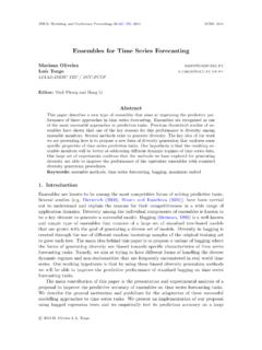
7 Choose by minimizing squared one-step prediction :Just a weighted moving be extended to include trend and intervals? Sort of ..Nate DerbyTime Series Forecasting Methods19 / 43 IntroductionUnivariate ForecastingConclusionsSeasonal Moving AverageExponential SmoothingARIMASAS CodeAll done withPROC FORECAST:method=expo trend=1for trend=2for seasons=( 12 )for 3 weeks ahead, exponential smoothingPROC FORECAST data=airline method=xx interval=month lead=12out=foreexsm outactual out1step;VAR pass;ID date;RUN;Nate DerbyTime Series Forecasting Methods20 / 43 IntroductionUnivariate ForecastingConclusionsSeasonal Moving AverageExponential SmoothingARIMA ! " " # $ % # & " '( )* + , " ! $ - " ./00/10200210300310400410100110500510600 0/7480/7100/71/0/7120/7130/7140/7110/715 0/7160/7190/7180/7500/75/0/752!"#$"%&'() **&%+&#*',)%-' ./.'0'1&2-' .3456789*)%:*'8;'<)**&%+&#*=Nate DerbyTime Series Forecasting Methods21 / 43 IntroductionUnivariate ForecastingConclusionsSeasonal Moving AverageExponential SmoothingARIMA !

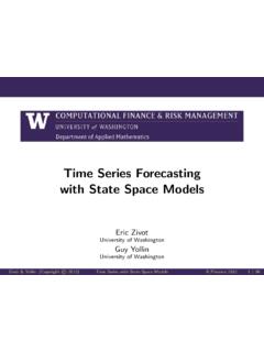
8 " " # $ % # & " '( )* + , " ! $ - " ./00/10200210300310400410100110500510600 0/7480/7100/71/0/7120/7130/7140/7110/715 0/7160/7190/7180/7500/75/0/752!"#$"%&'() **&%+&#*',)%-' ./.'0'1&2-' .345"6 7$ ")$'56 ::;<"%+'=:# *Nate DerbyTime Series Forecasting Methods22 / 43 IntroductionUnivariate ForecastingConclusionsSeasonal Moving AverageExponential SmoothingARIMA ! " " # $ % # & " '( )* + , " ! $ - " ./00/102002103003104004101001105005106000/7480/7100/71/0/7120/7130/7140/7110/7150/7160/7190/7180/7500/75/0/752!"#$"%&'()**&%+&#*',)%-' ./.'0'1&2-' .341567$ ")$'<= 55;>"%+'?5# *Nate DerbyTime Series Forecasting Methods23 / 43 IntroductionUnivariate ForecastingConclusionsSeasonal Moving AverageExponential SmoothingARIMA ! " " # $ % # & " '( )* + , " ! $ - " ./00/10200210300310400410100110500510600 0/7480/7100/71/0/7120/7130/7140/7110/715 0/7160/7190/7180/7500/75/0/752!"#$"%&'() **&%+&#*',)%-' ./.'0'1&2-' .345&)*6%)$'7896% 66:<"%+'=6#&2)*:*Nate DerbyTime Series Forecasting Methods24 / 43 IntroductionUnivariate ForecastingConclusionsSeasonal Moving AverageExponential SmoothingARIMAE xponential Smoothing VIAdvantages:Gives interpretable results (trend + seasonality).

9 Gives more weight to recent :Not a model (in the statistical sense).Prediction intervals not (really) t generalize to multivariate DerbyTime Series Forecasting Methods25 / 43 IntroductionUnivariate ForecastingConclusionsSeasonal Moving AverageExponential SmoothingARIMAARIMA IStands forAutoRegressive Integrated Moving known as Box-Jenkins models (Box and Jenkins, 1970).Advantages:Best fit (minimum mean squared forecast error).Generalizes to multivariate used :More intuitiveat DerbyTime Series Forecasting Methods26 / 43 IntroductionUnivariate ForecastingConclusionsSeasonal Moving AverageExponential SmoothingARIMAARIMA IIAssume nonseasonality for , transform, then difference the data{Yt}dtimes until itis stationary (constant mean, variance), denoted{Y t}.Guesstimate ordersp,qthrough the sample autocorrelation,partial autocorrelation anautoregressive moving average(ARMA) process,orderspandq:Y t 1Y t 1 pY t p=Zt+ 1Zt 1+ + qZt q (Y t) = (Zt)whereZtiid N(0, 2), and 1.

10 , p, 1,.., qare trial and error, repeat above 2 steps until errors lookgood .Above is an ARIMA(p,d,q) DerbyTime Series Forecasting Methods27 / 43 IntroductionUnivariate ForecastingConclusionsSeasonal Moving AverageExponential SmoothingARIMAC onfused Yet?Q: How do we account for seasonality, periods?A: We do almost the exact same thing, except for periods:Look at{Y t,Y t+s,Y t+2s,..}. Are they stationary? If not,differenceDtimes until they ordersPandQsimilarly to multiplicative ARMA(P,Q) process, periods:(Y t 1Y t s PY t Ps) (Y t) =(Zt+ 1Zt s+ + QZt Qs) (Zt)Repeat above 2 steps until all looks good .Above is an ARIMA(p,d,q)(P,D,Q) DerbyTime Series Forecasting Methods28 / 43 IntroductionUnivariate ForecastingConclusionsSeasonal Moving AverageExponential SmoothingARIMASAS CodeIf you re still with me ..Yt=log(passt) ARIMA(0,1,1) (0,1,1)12:(Yt Yt 1)(Yt Yt 12) = (Zt 1Zt 1)(Zt 1Zt 12) Forecasting 3 weeks ahead, ARIMAPROC ARIMA data=airline;IDENTIFY var=lpass( 1, 12 ) noprint;ESTIMATE q=( 1 )( 12 ) noint method=ML noprint;FORECAST lead=12 out=forearima id=date interval=month noprint;RUN;QUIT;Compare with Moving AverageNate DerbyTime Series Forecasting Methods29 / 43 IntroductionUnivariate ForecastingConclusionsSeasonal Moving AverageExponential SmoothingARIMA !