Transcription of Understanding Poles and Zeros 1 System Poles and Zeros
1 massachusetts institute OF technology . DEPARTMENT OF MECHANICAL ENGINEERING. Analysis and Design of Feedback Control Systems Understanding Poles and Zeros 1 System Poles and Zeros The transfer function provides a basis for determining important System response characteristics without solving the complete di erential equation. As de ned, the transfer function is a rational function in the complex variable s = + j , that is bm sm + bm 1 sm 1 + .. + b1 s + b0. H(s) = (1). an sn + an 1 sn 1 + .. + a1 s + a0. It is often convenient to factor the polynomials in the numerator and denominator, and to write the transfer function in terms of those factors: N (s) (s z1 )(s z2 ) .. (s zm 1 )(s zm ). H(s) = =K , (2). D(s) (s p1 )(s p2 ) .. (s pn 1 )(s pn ). where the numerator and denominator polynomials, N (s) and D(s), have real coe cients de ned by the System 's di erential equation and K = bm /an.
2 As written in Eq. (2) the zi 's are the roots of the equation N (s) = 0, (3). and are de ned to be the System Zeros , and the pi 's are the roots of the equation D(s) = 0, (4). and are de ned to be the System Poles . In Eq. (2) the factors in the numerator and denominator are written so that when s = zi the numerator N (s) = 0 and the transfer function vanishes, that is lim H(s) = 0. s zi and similarly when s = pi the denominator polynomial D(s) = 0 and the value of the transfer function becomes unbounded, lim H(s) = . s pi All of the coe cients of polynomials N (s) and D(s) are real, therefore the Poles and Zeros must be either purely real, or appear in complex conjugate pairs. In general for the Poles , either pi = i , or else pi , pi+1 = i j i . The existence of a single complex pole without a corresponding conjugate pole would generate complex coe cients in the polynomial D(s).
3 Similarly, the System Zeros are either real or appear in complex conjugate pairs. 1. Example A linear System is described by the di erential equation d2 y dy du 2. + 5 + 6y = 2 + 1. dt dt dt Find the System Poles and Zeros . Solution: From the di erential equation the transfer function is 2s + 1. H(s) = . (5). s2 + 5s + 6. which may be written in factored form 1 s + 1/2. H(s) =. 2 (s + 3)(s + 2). 1 s ( 1/2). = . (6). 2 (s ( 3))(s ( 2)). The System therefore has a single real zero at s = 1/2, and a pair of real Poles at s = 3 and s = 2. The Poles and Zeros are properties of the transfer function, and therefore of the di erential equation describing the input-output System dynamics. Together with the gain constant K they completely characterize the di erential equation, and provide a complete description of the System . Example A System has a pair of complex conjugate Poles p1 , p2 = 1 j2, a single real zero z1 = 4, and a gain factor K = 3.
4 Find the di erential equation representing the System . Solution: The transfer function is s z H(s) = K. (s p1 )(s p2 ). s ( 4). = 3. (s ( 1 + j2))(s ( 1 j2)). (s + 4). = 3 2 (7). s + 2s + 5. and the di erential equation is d2 y dy du 2. + 2 + 5y = 3 + 12u (8). dt dt dt 2. Figure 1: The pole - zero plot for a typical third-order System with one real pole and a complex conjugate pole pair, and a single real zero . The pole - zero Plot A System is characterized by its Poles and Zeros in the sense that they allow reconstruction of the input/output di erential equation. In general, the Poles and Zeros of a transfer function may be complex, and the System dynamics may be represented graphically by plotting their locations on the complex s-plane, whose axes represent the real and imaginary parts of the complex variable s. Such plots are known as pole - zero plots.
5 It is usual to mark a zero location by a circle ( ) and a pole location a cross ( ). The location of the Poles and Zeros provide qualitative insights into the response characteristics of a System . Many computer programs are available to determine the Poles and Zeros of a System from either the transfer function or the System state equations [8]. Figure 1. is an example of a pole - zero plot for a third-order System with a single real zero , a real pole and a complex conjugate pole pair, that is;. (3s + 6) (s ( 2)). H(s) = =3. (s3 2. + 3s + 7s + 5) (s ( 1))(s ( 1 2j))(s ( 1 + 2j)). System Poles and the Homogeneous Response Because the transfer function completely represents a System di erential equation, its Poles and Zeros e ectively de ne the System response. In particular the System Poles directly de ne the components in the homogeneous response.
6 The unforced response of a linear SISO System to a set of initial conditions is n . yh (t) = Ci e i t (9). i=1. where the constants Ci are determined from the given set of initial conditions and the exponents i are the roots of the characteristic equation or the System eigenvalues. The characteristic equation is D(s) = sn + an 1 sn 1 + .. + a0 = 0, (10). and its roots are the System Poles , that is i = pi , leading to the following important relationship: 3. Figure 2: The speci cation of the form of components of the homogeneous response from the System pole locations on the pole - zero plot. The transfer function Poles are the roots of the characteristic equation, and also the eigenvalues of the System A matrix. The homogeneous response may therefore be written n . yh (t) = Ci epi t . (11). i=1. The location of the Poles in the s-plane therefore de ne the n components in the homogeneous response as described below: 1.
7 A real pole pi = in the left-half of the s-plane de nes an exponentially decaying component , Ce t , in the homogeneous response. The rate of the decay is determined by the pole location; Poles far from the origin in the left-half plane correspond to components that decay rapidly, while Poles near the origin correspond to slowly decaying components. 2. A pole at the origin pi = 0 de nes a component that is constant in amplitude and de ned by the initial conditions. 3. A real pole in the right-half plane corresponds to an exponentially increasing component Ce t in the homogeneous response; thus de ning the System to be unstable. 4. A complex conjugate pole pair j in the left-half of the s-plane combine to generate a response component that is a decaying sinusoid of the form Ae t sin ( t + ) where A and are determined by the initial conditions.
8 The rate of decay is speci ed by ; the frequency of oscillation is determined by . 5. An imaginary pole pair, that is a pole pair lying on the imaginary axis, j generates an oscillatory component with a constant amplitude determined by the initial conditions. 4. 6. A complex pole pair in the right half plane generates an exponentially increasing component. These results are summarized in Fig. 2. Example Comment on the expected form of the response of a System with a pole - zero plot shown in Fig. 3 to an arbitrary set of initial conditions. Figure 3: pole - zero plot of a fourth-order System with two real and two complex conjugate Poles . Solution: The System has four Poles and no Zeros . The two real Poles correspond to decaying exponential terms C1 e 3t and C2 e , and the complex conjugate pole pair introduce an oscillatory component Ae t sin (2t + ), so that the total homogeneous response is yh (t) = C1 e 3t + C2 e + Ae t sin (2t + ) (12).
9 Although the relative strengths of these components in any given situation is determined by the set of initial conditions, the following general observations may be made: 1. The term e 3t , with a time-constant of seconds, decays rapidly and is signi cant only for approximately 4 or 2. The response has an oscillatory component Ae t sin(2t + ) de ned by the com- plex conjugate pair, and exhibits some overshoot. The oscillation will decay in approximately four seconds because of the e t damping term. 3. The term e , with a time-constant = 10 seconds, persists for approximately 40 seconds. It is therefore the dominant long term response component in the overall homogeneous response. 5. Figure 4: De nition of the parameters n and for an underdamped, second-order System from the complex conjugate pole locations. The pole locations of the classical second-order homogeneous System d2 y dy 2.
10 + 2 n + n2 y = 0, (13). dt dt described in Section are given by . p1 , p2 = n n 2 1. (14). If 1, corresponding to an overdamped System , the two Poles are real and lie in the left-half plane. For an underdamped System , 0 < 1, the Poles form a complex conjugate pair, . p1 , p2 = n j n 1 2 (15). and are located in the left-half plane, as shown in Fig. 4. From this gure it can be seen that the Poles lie at a distance n from the origin, and at an angle cos 1 ( ) from the negative real axis. The Poles for an underdamped second-order System therefore lie on a semi-circle with a radius de ned by n , at an angle de ned by the value of the damping ratio . System Stability The stability of a linear System may be determined directly from its transfer function. An nth order linear System is asymptotically stable only if all of the components in the homogeneous response from a nite set of initial conditions decay to zero as time increases, or n.