Transcription of Worked Examples in Dynamic Optimization: Analytic and ...
1 Worked Examples in Dynamic optimization : Analytic and numeric MethodsLaurent Cretegny Centre of Policy Studies, Monash University,AustraliaThomas F. Rutherford Department of Economics, University of ColoradoUSAM arch 29, 2004 AbstractEconomists are accustomed to think about economic growth models in con-tinuous time. However, applied models require numerical methods because ofthe absence of tractable analytical solutions. Since these methods operate byessence in discrete time, models involve discrete formulation. We demonstratethe usefulness of two off-the-shelf algorithms to solve these problems : nonlin-ear programming and mixed complementarity. We then show the advantageof the latter for approximating infinite-horizon classification:C69; D58; D91 Keywords: Dynamic optimization ; Mathematical methods; Infinite-horizonmodels Mailing address : Centre of Policy Studies, PO Box 11E, Monash University, Clayton Vic 3800,Australia.
2 E-mail: The author gratefully acknowledges financial supportfrom the Swiss National Science Foundation (post-doctoral research fellowship). Mailing address : Department of Economics, University of Colorado, Boulder, USA. IntroductionDynamic optimization in economics appeared in the 1920s with the work of Hotellingand Ramsey. In the 1960s Dynamic mathematical techniques became then more fa-miliar to economists mainly due to the work of neoclassical growth theorists. Thesetechniques involve most of the time formulation of models in continuous time. Whenclosed form solutions do not exist they are then formulated in discrete time. Thepurpose of this document is to provide some sample solutions of a collection ofdynamic optimization problems in two settings, using analytical methods in contin-uous time and numerical methods in discrete of infinite-horizon models are not possible with numerical approximation issues are crucial in finite-horizon models.
3 We consider twoclasses of off-the-shelf algorithms to solve these Dynamic models. The first is non-linear programming (NLP) developed originally for optimal planning models. Thesecond class is the mixed complementarity problem (MCP) approach. The MCPformulation is represented by the first-order conditions for nonlinear any NLP problem can be solved as an MCP formulation, not necessarily asefficient as using NLP-specific infinite-horizon models is illustrated in figure 1. The two innercircles represent the idea that the finite MCP formulation includes any of the NLPformulations. These two finite formulations are a subset of the infinite-horizon NLPformulation. It is then intuitively clear that an MCP formulation should provide a better approximation to infinite-horizon models than an NLP formulation.
4 Thecloseness of approximation is informally portrayed by the Euclidian distance in 1: Approximating infinite-horizon modelsThe outline of the paper is as follows. Starting from the classical mathematicaltechnique to solve Dynamic economizing problems in continuous time, the nextsection shows how to derive the NLP and MCP formulation to solve these 3 presents in detail analytical solutions to economic planning problems andshows how to formulate them in off-the-shelf softwares. The following section moveson to the neoclassical growth model. The last section explains how to use theoptimal neoclassical growth model in applied Mathematical MethodsThe Dynamic economizing problem may be solved in three different first approach going back up to Bernoulli in the very late 1600s is the calculusof variations.
5 The second is the maximum principal developed in the 1950s by Pon-tryagin and his co-workers. The third approach is Dynamic programming developedby Bellman about the same applications of Dynamic optimization to economics are due to Ramseyand Hotelling in the 1920s. At that time the mathematical technique used to solvedynamic problems was the calculus of variations. Therefore in the following sectionwe first state in a concise way the calculus of variations problem. Then we moveon to the maximum principle which can be considered a Dynamic generalization ofthe method of Lagrange multiplier. This method is well-known among economistsand is especially suited to the formulation in discrete time. Regarding dynamicprogramming it is usually applied to stochastic models and then will not be Continuous time approachThe classical calculus of variations problem may be written asmax{x(t)}J= t1t0I(x(t), x (t), t)dtsubject to various initial and endpoint conditionswhere these conditions are defined as equation:Fx=dFx /dt,t0 t condition:Fx x 0,t0 t conditions:- Initial conditions always apply:x(t0) = terminal time and terminal value may be fixed exogenously or conditions apply when the terminal value and time are free.
6 -If only the terminal value is free, thenFx = 0 only the terminal time is free, thenF x Fx = 0 both the terminal value and time are free, thenF= 0 andFx = 0 necessary conditions of the calculus of variations can be derived fromthe maximum principle. Intuitively it remains to let the rates of change of thestate variables to be the control variables in the maximum principle, which meansu(t) =x (t). Assuming that the terminal time value is fixed, which is always thecase in numerical problems, the corresponding maximum principle may be definedasmax{u(t)}J= t1t0I(x(t), u(t), t)dt+F(x(t1), t1)subject tox (t) =f(x(t), u(t), t)t0, t1andx(t0) =x0fixedx(t1) =g(x(t1), t1) or free2whereI( ) is the intermediate function,F( ) is the final function,f( ) is the stateequation function andg( ) is the terminal constraint a concise way the maximum principle technique involves adding costate vari-ables (t) to the problem, defining a new function called the Hamiltonian,H(x(t), u(t), (t), t) =I(x, u, t) + (t)f(x, u, t)and solving for trajectories{u(t)},{ (t)}, and{x(t)}
7 }satisfying the following con-ditionsoptimality condition H u=Iu+ fu= 0costate equation = H x= (Ix+ fx)state equationx = H =fwithx(t0) =x0terminal conditions x(t1) 0 (t1) F x (t1) = F x+ g xwith 0 x(t1) =g(x(t1), t1)which are necessary for a local Discrete time formulationThe formulation of the discrete time version of the maximum principle is straight-forward. Forming the Hamiltonian,H(xt, ut, t+1, t) =I(x, u, t) + t+1f(x, u, t)the necessary conditions are as follow:optimality condition H ut=Iu+ t+1fu= 0costate equation t+1 t= H xt= (Ix+ t+1fx)state equationxt+1 xt= H t+1=fwithxt0=x0terminal conditions xt1+1 0 t1+1 F x t1+1= F xt1+1+ g xt1+1with 0 xt1+1=g(xt1+1, t1+ 1)As mentioned earlier, the maximum principle can be considered the extensionof the method of Lagrange multipliers to Dynamic optimization problems.
8 Thismethod allows us to state problems in the same way they would be written in off-the-shelf softwares. WriteLfor the Lagrangian of the full intertemporal NLP formulation is thenmax{u(t)},{ (t)},{x(t)}L=t1 t=t0I(xt, ut, t) + t+1[xt+f(xt, ut, t) xt+1]+ t0[xt0 x0] + t1+1[g(xt1+1, t1+ 1) xt1+1] +F(xt1+1, t1+ 1)3and the MCP formulation follows from the first-order conditions L ut=Iu(xt, ut, t) + t+1fu(xt, ut, t) = 0t=t0, .. , t1 L xt=Ix(xt, ut, t) + t+1fx(xt, ut, t) + t+1 t= 0t=t0, .. , t1 L xt1+1= t1+1+ t1+1(gx 1) +Fx= 0 L t+1=f(xt, ut, t) (xt+1 xt) = 0t=t0, .. , t1 L t0=xt0 x0= 0 L t1+1=g(xt1+1, t1+ 1) xt1+1= 0which are the necessary conditions of the maximum method of Lagrange multipliers shows clearly that when the system has afixed final state, as here, there are two constraints for the terminal periodt1+1: thestate variablext1+1must satisfy the terminal constraint and still satisfies the stateequation.
9 This explains the two Lagrange multipliers associated withxt1+1: t1+1for the state equation, and t1+1for the terminal constraint. When the systemhas a free final state, which means that the terminal constraint is not specified, theLagrange multiplier t1+1is equal to zero if the value of the final function is Economic Planning Optimal consumption plan1 Find the consumption planC(t), 0 t T, over a fixed period to maximize thediscounted utility stream T0e rtCa(t)dtsubject toC(t) =iK(t) K (t), K(0) =K0, K(T) = 0where 0< a <1 andKrepresents the capital solutionWe have a variational problem based on the function:F(t, k, k ) =e rtU(ik k )Taking derivatives, we have:Fk=ie rtU andFk = e rtU The Euler equation is then:ddt[ e rtU ]=ie rtU 1 Problem in Kamien and Schwartz (2000).
10 4 Although the underlying problem is defined in terms of the capital stock, it isconvenient at this point to use consumption as the decision variable, when we formthe time derivative we have:re rtU e rtU c =ie rtU which reduces to: U c U =i rIn the case of constant elasticity utility,U(c) =ca,the Euler equation becomes:(1 a)c c=i rand, integrating we determine the growth rate of consumption:c=c0ei r1 atIn this expression, initial consumption level is a constant of integration. In orderto determine the consumption level, we need to focus on the initial and terminalconditions for the capital stock. To determine the time path of the capital stock, weconsider the equation which relates consumption to capital earnings and investment:ik k =c0ei r1 atIn order to solve an equation of this form, it is necessary to use a standard methodfor solving this sort of an equation, multiplying by an integrating factor:e it[k ik] = c0e tin which we define: =i r1 a i=ai r1 aThis equation can be written:d[e itk(t)]= c0e tdtwhich integrates to:e itk(t) = c0e t so:k(t) = eit c0 ei r1 atWe then have two boundary conditions to determine the constants of integration:k(0) =k0, k(T) = 0 The initial condition produces: =k0+c0 Substituting into the terminal condition, we have.