Transcription of www.stata.com
1 Exponential Single-exponential smoothingSyntaxMenuDescriptionOptionsRem arks and examplesStored resultsMethods and formulasReferencesAlso seeSyntaxtssmooth exponential[type]newvar=exp[if] [in] [,options]optionsDescriptionMainreplacer eplacenewvarif it already existsparms(# )use# as smoothing parametersamp0(#)use#observations to obtain initial value for recursions0(#)use#as initial value for recursionforecast(#)use#periods for the out-of-sample forecastYou musttssetyour data before usingtssmooth exponential; see [TS] contain time-series operators; see[U] Time-series >Time series>Smoothers/univariate forecasters>Single-exponential smoothingDescriptiontssmooth exponentialmodels the trend of a variable whose change from the previous valueis serially correlated.
2 More precisely, it models a variable whose first difference follows a low-order,moving-average Main replacereplacesnewvarif it already (# )specifies the parameter for the exponential smoother;0<# <1. Ifparms(# )is not specified, the smoothing parameter is chosen to minimize the in-sample sum-of-squaredforecast (#)ands0(#)are mutually exclusive ways of specifying the initial value for the (#)specifies that the initial value be obtained by calculating the mean over the first#observations of the (#)specifies the initial value to be neither option is specified, the default is to use the mean calculated over the first half of (#)gives the number of observations for the out-of-sample prediction;0 # 500.
3 Thedefault value isforecast(0)and is equivalent to not forecasting out of tssmooth exponential Single-exponential smoothingRemarks and of missing valuesIntroductionExponential smoothing can be viewed either as an adaptive-forecasting algorithm or, equivalently,as a geometrically weighted moving-average filter. Exponential smoothing is most appropriate whenused with time-series data that exhibit no linear or higher-order trends but that do exhibit low-velocity, aperiodic variation in the mean. Abraham and Ledolter (1983), Bowerman, O Connell, andKoehler (2005), and Montgomery, Johnson, and Gardiner (1990) all provide good introductions tosingle-exponential smoothing.
4 Chatfield (2001, 2004) discusses how single-exponential smoothingrelates to modern time-series methods. For example, simple exponential smoothing produces optimalforecasts for several underlying models, includingARIMA(0,1,1) and the random-walk-plus-noisestate-space model. (See Chatfield [2001, sec. ].)The exponential filter with smoothing parameter creates the seriesSt, whereSt= Xt+ (1 )St 1fort= 1,..,TandS0is the initial value. This is the adaptive forecast-updating form of the exponential implies thatSt= T 1 k=0(1 )KXT k+ (1 )TS0which is the weighted moving-average representation, with geometrically declining weights.
5 Thechoice of the smoothing constant determines how quickly the smoothed series or forecast will adjustto changes in the mean of the unfiltered series. For small values of , the response will be slowbecause more weight is placed on the previous estimate of the mean of the unfiltered series, whereaslarger values of will put more emphasis on the most recently observed value of the unfiltered 1: Smoothing a series for specified parametersLet s consider some examples using sales data. Here we forecast sales for three periods with asmoothing parameter of :. use tssmooth exponential sm1=sales, parms(.4) forecast(3)exponential coefficient = residuals = 8345root mean squared error = compare our forecast with the actual data, we graph the series and the forecasted series exponential Single-exponential smoothing 3.
6 Line sm1 sales t, title("Single exponential forecast")> ytitle(Sales) xtitle(Time)100010201040106010801100 Sales01020304050 Timeexp parms( ) = salessalesSingle exponential forecastThe graph indicates that our forecasted series may not be adjusting rapidly enough to the changesin the actual series. The smoothing parameter controls the rate at which the forecast values of adjust the forecasts more slowly. Thus we suspect that our chosen value of too small. One way to investigate this suspicion is to asktssmooth exponentialto choose thesmoothing parameter that minimizes the sum-of-squared forecast tssmooth exponential sm2=sales, forecast(3)computing optimal exponential coefficient (0,1)optimal exponential coefficient = residuals = mean squared error = output suggests that the value of = is too small.
7 The graph below indicates that thenew forecast tracks the series much more closely than the previous line sm2 sales t, title("Single exponential forecast with optimal alpha")> ytitle(sales) xtitle(Time)100010201040106010801100 Sales01020304050 Timeparms( ) = salessalesSingle exponential forecast with optimal alpha4 tssmooth exponential Single-exponential smoothingWe noted above that simple exponential forecasts are optimal for anARIMA(0,1,1) model. (See[TS]arimafor fittingARIMA models in Stata.) Chatfield (2001, 90) gives the following usefulderivation that relates theMAcoefficient in anARIMA(0,1,1) model to the smoothing parameter insingle-exponential smoothing.
8 AnARIMA(0,1,1) is given byxt xt 1= t+ t 1where tis an identically and independently distributed white-noise error term. Thus given , anestimate of , an optimal one-step prediction of xt+1is xt+1=xt+ t. Because tis not observable,it can be replaced by t=xt xt 1yielding xt+1=xt+ (xt xt 1)Letting = 1 + and doing more rearranging implies that xt+1= (1 + )xt xt 1 xt+1= xt (1 ) xt 1 Example 2: Comparing ARIMA to exponential smoothingLet s compare the estimate of the optimal smoothing parameter of with the one we couldobtain using [TS]arima. Below we fit anARIMA(0,1,1) to the sales data and then remove the estimateof . The two estimates of are quite close, given the large estimated standard error of.
9 Arima sales, arima(0,1,1)(setting optimization to BHHH)Iteration 0: log likelihood = 1: log likelihood = 2: log likelihood = 3: log likelihood = 4: log likelihood = (switching optimization to BFGS)Iteration 5: log likelihood = regressionSample: 2 - 50 Number of obs = 49 Wald chi2(1) = likelihood = Prob > chi2 = Std. Err. z P>|z| [95% Conf. Interval] .1671699 .1289908 : The test of the variance against zero is one sided, and the two-sidedconfidence interval is truncated at di 1 + _b[ ].
10 80134387tssmooth exponential Single-exponential smoothing 5 Example 3: Handling panel datatssmooth exponentialautomatically detects panel data. Suppose that we had sales figures forfive companies in long form. Runningtssmooth exponentialon the variable that contains all fiveseries puts the smoothed series and the predictions in one variable in long form. When the smoothingparameter is chosen to minimize the squared prediction error, an optimal value for the smoothingparameter is chosen separately for each use , clear. tssetpanel variable: id (strongly balanced)time variable: t, 1 to 100delta: 1 unit. tssmooth exponential sm5=sales, forecast(3)-> id = 1computing optimal exponential coefficient (0,1)optimal exponential coefficient = residuals = mean squared error = > id = 2computing optimal exponential coefficient (0,1)optimal exponential coefficient = residuals = mean squared error = > id = 3computing optimal exponential coefficient (0,1)optimal exponential coefficient = residuals = 21629root mean squared error = > id = 4computing optimal exponential coefficient (0,1)