17: Transmission Lines

6: Operational Amplifiers

6: Operational Amplifiers 6: Operational Amplifiers •Operational Amplifier •Negative Feedback •Analysing op-amp circuits •Non-inverting amplifier •Voltage Follower

  Operational, Amplifiers, Operational amplifiers, Operational amplifiers 6

FINANCIAL REGULATIONS PREAMBLE

1 FINANCIAL REGULATIONS PREAMBLE 1.1 These Regulations are made by the Director of Finance, acting on the advice of the Management Board, under powers conferred by the Council under paragraph 5 of Ordinance C1.

  Regulations, Financial, Preamble, Financial regulations preamble

Convolution Table (1) Convolution Table (2)

with System’s impulse response h(t). Convolution Integral ... weighted by h(t- τ) (i.e. x(τ) h(t- τ)) for the shaded pulse, PLUS the contribution from all the previous pulses of x(τ). The summation of all these weighted inputs is the convolution integral. L2.4-2 p191

  Convolutions

Signal Transmission through LTI Systems

PYKC 20-Feb-11 E2.5 Signals & Linear Systems Lecture 12 Slide 9 Parseval’s Theorem The energy of a signal x(t) can be derived in time or frequency domain:

  Transmissions, Signal, Theorem, Parseval s theorem, Parseval, Signal transmission

Tutorial 7 - Sampling

PYKC – 11 Feb 08 2 E2.5 Signals & Linear Systems Tutorial Sheet 7 – Sampling (Lectures 12 - 13) 1.* By applying the Parseval’s theorem, show that

  Sampling, Theorem, Parseval s theorem, Parseval, 7 sampling

Lecture 8 - Timing Constraints

Metastability is a problem that arises when an external input NOT synchronised to the system clock is fed into our synchronous circuit. Since the input signal could change anytime relative the the clock edge, metastability will occur. It could also happens when a signal crosses from one clock domain (Clock1) to another clock domain (Clock2).

  Metastability

14: Power in AC Circuits

Cosine Wave RMS 14: Power in AC Circuits •Average Power •Cosine Wave RMS •Power Factor + •Complex Power •Power in R, L, C •Tellegen’s Theorem •Power Factor Correction •Ideal Transformer •Transformer Applications •Summary E1.1 Analysis of Circuits (2017-10213) AC Power: 14 – 3 / 11 Cosine Wave: v(t) = 5cosωt.Amplitude is V = 5V. Squared Voltage: v2(t) = …

SERVO MOTOR SG90 DATA SHEET - Imperial College London

SERVO MOTOR SG90 DATA SHEET Tiny and lightweight with high output power. Servo can rotate approximately 180 degrees (90 in each direction), and works just like the standard kinds but smaller. You can use any servo code, hardware or library to control these servos.

  Sheet, Data, Motor, Data sheet, Servo, Servo motors

8: Correlation - Imperial College London

E1.10 Fourier Series and Transforms (2015-5585) Fourier Transform - Correlation: 8 – 3 / 11 Cross correlation is used to find where two signals match: u(t) is the test waveform.

  Tests, Correlations

3: Nodal Analysis

We assume the interconnections have zero resistance so all points within a node have the same voltage. Five nodes: A,···,E. Ohm’s Law: VBD = IR5 KVL: VBD = VB −VD KCL: Total current exiting any closed region is zero.

  Interconnection

RF and Microwave Power Amplifier Design

Transmission Line 21 Chapter 2. Nonlinear Circuit Design Methods 27 Spectral Domain Analysis 27 Trigonometric identities 28 Piecewise-linear approximation 29 Bessel functions 33 Time Domain Analysis 35 Newton-Raphson Algorithm 42 Quasilinear Method 45 Harmonic Balance Method 48 Chapter 3. Nonlinear Active Device Modeling 53 Power MOSFETs 54

  Line, Transmissions, Transmission line

III. Three-Phase Circuits

2. Connection Types There are two types of connections in three-phase circuits: Y (Wye) and Δ(Delta) Each generator and each load can be either Y-or Δ-connected.Any number of Y- and Δ-connected elements may be mixed in a power system. Phase quantities – voltages and currents in a given phase. Line quantities – voltages between the lines and currents in the lines connected

  Phases, Line, Circuit, Three, Three phase circuits

Lecture -- Transmission Line Equations - EMPossible

Transmission Line Equations Lecture Outline •Introduction •Transmission Line Equations •Transmission Line Wave Equations Slide 2 1 2. 9/21/2019 2 Slide 3 Introduction Map of Waveguides (LI Media) Slide 4 Transmission Lines •Contains two or more conductors.

  Lecture, Line, Transmissions, Equations, Transmission line, Transmission line equations, Lecture transmission line equations, Transmission line equations lecture

Lectures on Electromagnetic Field Theory

Dec 04, 2019 · 15.2 Homomorphism of Uniform Plane Waves and Transmission Lines Equations . 148 1 These polarizations are also variously know as the sand ppolarizations, a descendent from the notations for acoustic waves where sand pstand for shear and pressure waves respectively.

  Lecture, Field, Transmissions, Theory, Equations, Electromagnetic, Lectures on electromagnetic field theory

Lecture 11 Transmission Lines - Purdue University

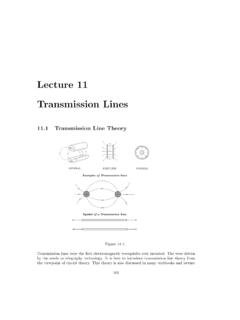
Lecture 11 Transmission Lines 11.1 Transmission Line Theory Figure 11.1: Transmission lines were the rst electromagnetic waveguides ever invented. The were driven by the needs in telegraphy technology. It is best to introduce transmission line theory from the viewpoint of circuit theory. This theory is also discussed in many textbooks and ...

  Lecture, Line, Transmissions, Transmission line

Power System Analysis

equations harder to solve. For the solution of the equations, the linearization ∂f ∂x ∆x = ∆y (1.2) is quite often used and solved. These equations give also very useful infor-mation about the system. The Jacobian matrix ∂f ∂x, whose elements are given by ∂f ∂x ij = ∂f i ∂x j (1.3)

  Equations

Numerical Methods for Partial Differential Equations

this lecture note is to provide students a convenient textbook that addresses both physical and mathematical aspects of numerical methods for partial dif-ferential equations (PDEs). In solving PDEs numerically, the following are essential to consider: •physical laws governing the differential equations (physical understand-ing),

  Lecture, Methods, Differential, Equations, Numerical, Partial, Ferential, Numerical methods for partial differential equations, Numerical methods for partial dif ferential equations

OPTICAL FIBER COMMUNICATION - SLAC

Starting from Maxwell equations: - Wave equation in cylindrical coordinates is derived. - The wave equation can be exactly solved for uniformly cored fibers. - The classification of type of solutions lead to TE, EH, or EH and HE modes. - For graded index non-uniform core profiles, approximate methods can be used.

  Communication, Optical, Brief, Equations, Optical fiber communication