Classification and regression trees
neighbor models in the nodes. GUIDE also can pro-duce ensemble models using bagging16 and random forest17 techniques. Table 1 summarizes the features of the algorithms. To see how the algorithms perform in a real ap-plication, we apply them to a data set on new cars for the 1993 model year.18 There are 93 cars and 25 variables.
Download Classification and regression trees

Information
Domain:
Source:
Link to this page:
Documents from same domain
P(Z Cumulative Probabilities of the Standard …
pages.stat.wisc.eduCumulative Probabilities of the Standard Normal Distribution N(0, 1) Left-sided area Left-sided area Left-sided area Left-sided area Left-sided area Left-sided area
BASIC CALCULUS REFRESHER - pages.stat.wisc.edu
pages.stat.wisc.edu3 y = x y = x2 Notice that the line has the generic equation y = f (x) = mx + b, where b is the Y-intercept (in this example, b = +3), and m is the slope of the line (in this example, m = +2). In general, the slope of any line is defined as the ratio of “height change” y to “length change” x, that is, m = y

Solutions to Homework 5 Statistics 302 Professor Larget
pages.stat.wisc.eduSolutions to Homework 5 Statistics 302 Professor Larget Textbook Exercises 4.79 Divorce Opinions and Gender In Data 4.4 on page 227, we introduce the results of a May 2010 Gallup poll of 1029 US adults. When asked if they view divorce as \morally acceptable", 71% of the men and 67% of the women in the sample responded yes. In the test for a di ...
Using lme4: Mixed-Effects Modeling in R
pages.stat.wisc.eduDe nition of linear mixed-e ects models A mixed-e ects model incorporates two vector-valued random variables: the response, Y, and the random e ects, B. We observe the value, y, of Y. We do not observe the value of B. In a linear mixed-e ects model the conditional distribution, YjB, and the marginal distribution, B, are independent,
Applications of Fourier Transform to Imaging Analysis
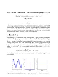
pages.stat.wisc.eduCallosum (CC) data are used to demonstrate the advantages of our method over previous methods. The possibilities of applications of this method to image analysis is discussed. 1 Introduction Fourier transform (FT) is named in the honor of Joseph Fourier (1768-1830), one of greatest names in the history of mathematics and physics.

Solutions to Homework 1 Statistics 302 Professor Larget
pages.stat.wisc.eduselected. Other options are possible: for example, we could number the plants from 1 to 30000 and randomly select 30 numbers between 1 and 30000. (b) Answers will vary for this question, but the procedure should be explained and the three numbers which were obtained should be listed. Here is the start of one sample. Row Plant #94 #180 #83 # 81 ...

3. The Gaussian kernel
pages.stat.wisc.eduThe Gaussian kernel is defined in 1-D, 2D and N-D respectively as ... process of observation s can never become zero. For, this would imply making an observation through an infinitesimally small aperture, which is impossible. The factor of 2 in the exponent is a matter of convention,

CHAPTER 8. RANDOMIZED COMPLETE BLOCK DESIGN …
pages.stat.wisc.eduMSEB is the mean square of design-B with degrees of freedom dfB. If RE>1, design A is more efficient. If RE<1, the converse is true. If a randomized complete block design (say, design-A) is used, one may want to estimate the relative efficiency compared with a completely randomized design (say, design-B).
Practice Exam Questions; Statistics 301; Professor Wardrop
pages.stat.wisc.edu13. A sample space has three possible outcomes, B, C, and D. It is known that P(C) = P(D). The operation of the chance mechanism is simulated 10,000 times (runs). The sorted frequencies of the three outcomes (B, C, and D) are: 2322, 2360, and 5318. (a) What is your approximation of P(B)? To receive credit you must explain your an-swer.
Power and Sample Size Determination
pages.stat.wisc.eduPower and Sample Size Determination Bret Hanlon and Bret Larget Department of Statistics University of Wisconsin|Madison November 3{8, 2011 Power 1 / 31 Experimental Design To this point in the semester, we have largely focused on methods to analyze the data that we have with little regard to the decisions on how to gather the data.
Related documents
A.1 SAS EXAMPLES
users.stat.ufl.edumodels using ML or Bayesian methods, cumulative link models for ordinal responses, zero-in ated Poisson regression models for count data, and GEE analyses for marginal models. PROC LOGISTIC gives ML tting of binary response models, cumulative link models for ordinal responses, and baseline-category logit models for nominal responses.

Maximum Likelihood Estimation of Logistic Regression ...
czep.netMaximum Likelihood Estimation of Logistic Regression Models 2 corresponding parameters, generalized linear models equate the linear com-ponent to some function of the probability of a given outcome on the de-pendent variable. In logistic regression, that function is the logit transform: the natural logarithm of the odds that some event will occur.
Logit Models for Binary Data
data.princeton.eduLogit Models for Binary Data We now turn our attention to regression models for dichotomous data, in-cluding logistic regression and probit analysis. These models are appropriate when the response takes one of only two possible values representing success and failure, or more generally the presence or absence of an attribute of interest.

Introduction to Binary Logistic Regression
wise.cgu.edu17 Binary logistic regression 21 Hierarchical binary logistic regression w/ continuous and categorical predictors 23 Predicting outcomes, p(Y=1) for individual cases 24 Data source, reference, presenting results 25 Sample results: write-up and table 26 How to graph logistic models with Excel 27 Plot of actual data for comparison to model 28 How ...

An Introduction to Logistic Regression Analysis and Reporting
datajobs.comLogistic Regression Models The central mathematical concept that underlies logistic regression is the logit—the natural logarithm of an odds ratio. The simplest example of a logit derives from a 2 ×2 contingency table. Consider an instance in which the distri- ... If a predictor is binary, as in the Table 1 example, then the odds ratio is ...

Logistic Regression in Rare Events Data
gking.harvard.eduFirst, although the statistical properties of linear regression models are invariant to the (unconditional) mean of the dependent variable, the same is not true for binary dependent variable models. The mean of a binary variable is the relative frequency of events in the

Multinomial Logistic Regression Models
socialwork.wayne.edusequence of binary models. In some cases, it makes sense to “factor” the response into a sequence of binary choices and model them with a sequence of ordinary logistic models. For example, consider the study of the effects of radiation exposure on mortality. The four-level response can be modeled in three stages: Population Alive Dead Non ...

Hierarchical Models - Princeton University
www.cs.princeton.edu• The two regression models everyone has heard of are – Linear regression for continuous responses, yi jxi »N (fl >x i,¾ 2) (6) – Logistic regression for binary responses (e.g., spam classification), p(yi ˘1jxi)˘logit(fl>xi) (7) – In both cases, the distribution of the response is governed by the linear combina-

An Introduction to Logistic and Probit Regression Models
www.liberalarts.utexas.eduModeling a Binary Outcome • Latent Variable Approach • We can think of y* as the underlying latent propensity that y=1 • Example 1: For the binary variable, heart attack/no heart attack, y* is the propensity for a heart attack. • Example 2: For the binary variable, in/out of the labor force, y* is the propensity to be in the labor force. ...

11 Logistic Regression - Interpreting Parameters
www.unm.edu11 LOGISTIC REGRESSION - INTERPRETING PARAMETERS 11 Logistic Regression - Interpreting Parameters Let us expand on the material in the last section, trying to make sure we understand the logistic regression model and can interpret Stata output. Consider first the case of a single binary predictor, where x = (1 if exposed to factor 0 if not;and y =