Convolution solutions (Sect. 6.6). Convolution of two ...

Thomas Calculus; 12th Edition: The Power Rule

Thomas Calculus; 12th Edition: The Power Rule Cli ord E. Weil September 15, 2010 The following paragraph appears at the bottom of page 116 of Thomas Calculus, 12th Edition. The Power Rule is actually valid for all real numbers n.

  Power, Edition, Thomas, Calculus, The power, 12th, Thomas calculus 12th edition, 12th edition, Thomas calculus

Convolution solutions (Sect. 6.6). - users.math.msu.edu

Convolution solutions (Sect. 6.6). I Convolution of two functions. I Properties of convolutions. I Laplace Transform of a convolution. I Impulse response solution. I Solution decomposition theorem.

Special Second Order Equations (Sect. 2.2). Special Second ...

Special Second Order Equations (Sect. 2.2). I Special Second order nonlinear equations. I Function y missing. (Simpler) I Variable t missing. (Harder) I Reduction order method. Special Second order nonlinear equations Definition Given a functions f : R3 → R, a second order differential equation in the unknown function y : R → R is given by

  Second, Special, Order, Equations, Sect, Second order, Special second order equations, Special second order

second order equations{Undetermined Coe - cients

September 29, 2013 9-1 9. Particular Solutions of Non-homogeneous second order equations{Undetermined Coe -cients We have seen that in order to nd the general solution to

  Second, Order, Equations, Undetermined, Second order equations undetermined

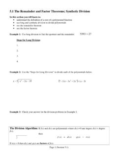
5.1 The Remainder and Factor Theorems.doc; Synthetic Division

Page 2 (Section 5.1) Example 4: Perform the operation below. Write the remainder as a rational expression (remainder/divisor). 2 1 2 8 2 3 5 4 3 2 + − + + x x x x x Synthetic Division – Generally used for “short” division of polynomials when the divisor is in the form x – c. (Refer to page 506 in your textbook for more examples.)

  Factors, Theorem, Remainder, The remainder and factor theorems

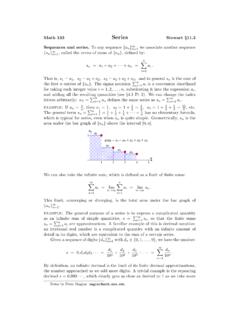
Math 133 Series Sequences and series. fa g

Geometric sequences and series. A general geometric sequence starts with an initial value a 1 = c, and subsequent terms are multiplied by the ratio r, so that a n = ra n 1; explicitly, a n = crn 1. The same trick as above gives a formula for the corresponding geometric series. We have s …

  Series, Sequence, Geometric, Geometric sequences and series, Geometric series, Series sequences and series

The Laplace Transform (Sect. 6.1). - users.math.msu.edu

The Laplace Transform (Sect. 6.1). I The definition of the Laplace Transform. I Review: Improper integrals. I Examples of Laplace Transforms. I A table of Laplace Transforms. I Properties of the Laplace Transform. I Laplace Transform and differential equations.

  Transform, Laplace transforms, Laplace, The laplace transform

ORDINARY DIFFERENTIAL EQUATIONS

The equations in examples (c) and (d) are called partial di erential equations (PDE), since the unknown function depends on two or more independent variables, t, x, y, and zin these examples, and their partial derivatives appear in the equations.

  Differential, Equations, Variable, Ordinary, Ordinary differential equations

Sequences and Series - Michigan State University

2 2. Sequences and Series A topological way to say lima n = ais the following: Given any -neighborhood V (a) of a, there exists a place in the sequence after which all of the terms are in V (a): Easy Fact: lim(c) = cfor all constant sequences (c): Quanti ers. The de nition of lima n = aquanti es the closeness of a n to aby an arbi-

  Series, Sequence, Sequences and series

Convergence of Taylor Series (Sect. 10.9) Review: Taylor ...

Convergence of Taylor Series (Sect. 10.9) I Review: Taylor series and polynomials. I The Taylor Theorem. I Using the Taylor series. I Estimating the remainder. The Taylor Theorem Remark: The Taylor polynomial and Taylor series are obtained from a generalization of the Mean Value Theorem: If f : [a,b] → R is differentiable, then there exits c ∈ (a,b) such that

  Review, Convergence

Time Response of Second Order Systems - Mercer University

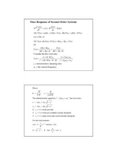
Impulse response of the second order system: Laplace transform of the unit impulse is R(s)=1 Impulse response: Transient response for the impulse function, which is simply is the derivative of the response to the unit step: ( 2) 2 2 2 n n n s s Y s ζω ω ω + + = y(t) e sin(n t)n n t ω β β = ω −ζω Responses and pole locations Time Responses and Pole Locations:

  Response, Impulse, Impulse response

5Properties of Linear, Time-Invariant Systems

vertible, then the impulse response hi of the inverse system has the property that h convolved with hi is an impulse. For LTI systems an equivalent condi-tion to stability is that the impulse response be absolutely summable (discrete time) or absolutely integrable (continuous time). If an LTI system is causal,

  Response, Impulse, Impulse response

AP Physics C: Mechanics - College Board

PHYSICSC: MECHANICS FREE-RESPONSE QUESTIONS : 2. Two carts are on a horizontal, level track of negligible friction. Cart 1 has a sensor that measures the force exerted on it during a collision with cart 2, which has a spring attached. Cart 1 is moving with a speed of : v : 0 =3.00 m s toward cart 2, which is at rest, as shown in the figure above.

  Physics, Response, Ap physics c

Impulse Response and Convolution

Impulse Response If a system is linear and time-invariant (LTI), its input-output relation is completely speci ed by the system’s impulse response h(t). 1. One can always nd the impulse response of a system. δ (t)system h 2. Time invariance implies that shifting the input simply shifts the output. δ (t−τ)system h 3.

  Response, Impulse, Impulse response

Modeling an Impulse in Simulink

Modeling an Impulse in Simulink INTRODUCTION Often a dynamic system is subject to an impulsive load, such as a blow from a hammer. It is important to be able to model such systems to understand what the response will be. This tutorial will discuss three methods for modeling an impulse in Simulink so that it can be used as the

  Response, Impulse