Transcription of Calculation of PCB Track Impedance
1 1 Calculation of PCB Track ImpedancebyAndrew J Burkhardt, Christopher S Gregg and J Alan StaniforthINTRODUCTIONThe use of high-speed circuits requires PCB tracks to bedesigned with controlled (characteristic, odd-mode, ordifferential) impedances. Wadell[1] is one of the mostcomprehensive sources of equations for evaluating theseimpedances. This source includes many configurationsincluding stripline, surface microstrip, and their IPC publication, IPC-2141[2], is another source ofequations but has a smaller range of configurations, similarto those presented in , for some configurations there are differencesbetween the equations given in these publications.
2 Theauthors believe that it is now opportune to examine theorigin of the equations and to update the method ofcalculation for use with modern personal an example, consider the surface microstrip shown inFigure 1 - Surface MicrostripIPC-2141[2] gives the characteristic Impedance as() ++= (1)Wadell[1] gives()() +++=2121' (2)where' += (3a) ++= rAB(3b)with''www +=(3c)The parameter w' is the equivalent width of a Track of zerothickness due to a Track of rectangular profile, width w andthickness t. Wadell[1] gives an additional equation todetermine the incremental value w'. The parameter o, inequation (2), is the Impedance of free-space (or vacuum), ( 120 ).
3 The quoted accuracy is 2% for any valueof r and 1 shows the results of applying equations (1) and (2)to a popular surface microstrip constructed from 1oz coppertrack on 1/32 inch 1 Equation (1)Equation (2)Widthw( m)NumericalMethodZ0 ( )Z0 ( )% errorZ0 ( )% + + = 35 m, h = 794 m, r = (the Calculation of the error assumes the numerical methodis accurate : see Numerical Results)Table 1 shows that equation (2) is well within the quotedaccuracy. The accuracy of equation (1) varies widely, butthis equation has the advantage of simplicity and is useful inillustrating the general changes to the value of Z0 as thewidth w and thickness t are example demonstrated by Table 1, highlights thegeneral problem with published equations: complicatedequations are usually more accurate.
4 Ranges over which theequations are accurate are also usually restricted to a limitedrange of parameters ( w/h, t/h and r).Equation (2) is complicated, but with patience, can beevaluated using a programmable calculator or computerSubstrateDielectric constant rwht2spreadsheet. However the complications increase greatlywhen two coupled tracks are used to give a differentialimpedance. For coupled surface microstrip, Wadell[1] gives7 pages of equations to evaluate the is now a major exercise to evaluate the Impedance using acalculator or EQUATIONSS ingle TrackFor the stripline of Figure 2 with a symmetrically centredtrack of zero thickness, Cohn[3] has shown that the exactvalue of the characteristic Impedance is()()' =(4)where = (5a)and = ' (5b)K is the complete elliptic function of the first kind[4].
5 Anequation for the evaluation of the ratio of the ellipticfunctions, accurate to 10-12, has been given by Hilberg[5],and also quoted by Wadell[1].Figure 2 - Stripline: Centred TrackWhen the thickness is not zero, corrections have to be madewhich are approximate[1]. These corrections are obtainedfrom theoretical approximations or curve fitting the resultsof numerical calculations based on the fundamentalelectromagnetic field the Track is offset from the centre, the publishedequations become more complicated and the range ofvalidity, for a given accuracy, is have also been made to include the effects ofdifferential etching on the Track resulting in a Track cross-section which is trapezoidal[1].
6 There is no closed-form equation like equation (4) forsurface or embedded microstrip of any Track any equation used to calculate the Impedance isapproximate and demonstrated in Table Coplanar TracksFigure 3 shows two coupled coplanar centred 3 - Stripline : CoplanarCoupled Centred TracksAll the Impedance equations for coupled configurationsrefer to both even-mode Impedance (Z0e) and odd-modeimpedance (Z0o). These impedances are measured betweenthe tracks and the ground plane. Z0e occurs when tracks Aand B are both at +V relative to the ground plane, and Z0ooccurs when Track A is at +V and Track B is at V. When adifferential signal is applied between A and B, then avoltage exists between the tracks similar to the odd-modeconfiguration.
7 The Impedance presented to this signal isthen the differential Impedance ,odiffZZ02 =(6)All published equations [1] give Z0o. The differentialimpedance must then be obtained using equation (6).For the zero thickness configuration of Figure 3, Cohn[3]gives the exact expression.()()0000' =(7)where()21200'1kk =(8a)and() + = '0 (8b)As before K is the elliptic function of the first kind. Thereare no closed-form equations for coplanar coupled of Track ThicknessWhen the Track thickness is not zero, approximations mustbe made to obtain algebraic equations similar to equations(4) and (7). Alternatively, equations, based on curve fittingof extensive numerical calculations, are , as the thickness increases the impedancedecrease, as can be noted from equation (1).
8 Substrate rwhwsBASubstrate rwh3 NUMERICAL PRINCIPLESFor pulses on a uniform transmission system,[1,6] then()CLZorZo=00(9)where L is the inductance and C the capacitance per unitlength of a stripline, where the electric (and magnetic) fields arein a uniform substrate, dielectric constant r, equation (9)becomescCZr =0(10)where c is the velocity of light in vacuuo (or free-space).The velocity of pulse travel along the transmission path isrc =(11)For a microstrip, the electric (and magnetic) fields are in airand the substrate, It can be shown thatairCCcZ10=(12)Where Cair is the capacitance of the same trackconfiguration without substrate. The effective dielectricconstant isaireffCC= (13)To find the Impedance , the capacitance must be can be done by applying a voltage V to the tracks andcalculating the total charge per unit length Q, from whichVQC=(14)However the surface charge on a Track is not uniform.
9 Infact it is very high at Track corners. Therefore the totalcharge is difficult to electrostatic theory, it is known that a charge producesa voltage at a distance r from the charge. Then adistribution of charge (coulomb/unit width of Track ) givesa voltage =lGV (15)where the integral is taken over the perimeter of the trackcross-section, l is a small length, and G is the voltage dueto a unit charge. It is also known as the Green s value of G depends on the configuration (orenvironment). For instance, a point charge in a 2dimensional dielectric space, without conductors gives()rrV 02ln =(16a)so that()rrG 02ln =(16b)In equation (15), the voltage V is known, G is known for theparticular configuration of tracks and substrate, but thecharge is unknown.
10 Thus (15) is an integral equationwhich can be solved numerically by the Method ofMoments (MoM)[7].To proceed using MoM, the cross-section perimeter of thetrack is divided into short lengths with a node at each are assigned to each node. The voltage at eachnode is calculated from all the nodal charges and theestimated charge variation between nodes. This leads to aset of simultaneous equations represented by the matrixequationVA= (17)where is a vector of nodal charges, and V is a vector ofnodal voltages. A is a square matrix whose elements arecalculated from integrals involving the Green s size of the matrices depends on the number of (17) can be solved for the nodal charges forgiven nodal voltages V.