Classic Transmission Line Enclosure Alignment Tables

1 Classic Transmission line Enclosure Alignment Tables Martin J. King 40 Dorsman Dr. Clifton Park, NY 12065. Classic Transmission line Enclosure Alignment Tables By Martin J. King, 10/16/03 (revised 10/20/06). Copyright 2003 by Martin J. King. All Rights Reserved. Introduction : Ever since I first made my original MathCad Transmission line worksheets available, the subject of Alignment Tables has come up again and again. Reasons vary;. some people had difficulty using the worksheets while others just wanted a starting geometry for input into the worksheets. When you design your first Transmission line Enclosure using the MathCad worksheets, it can be a little hard to get started. Learning how to use MathCad while also learning a new Enclosure design methodology is not easy for everybody. People are comfortable with the commonly available Alignment Tables for closed and ported enclosures. Box size and tuning frequency are expressed as functions of a driver's Thiele / Small parameters.

2 Alignment Tables represent a cookbook process with predictable results for designing closed or ported enclosures. Similar general Alignment Tables for Transmission line enclosures would allow quick scoping analyses of Enclosure geometries for different drivers under consideration. The scoping calculations could become the basis of a final design or the starting point for further optimization using the MathCad worksheets. As I continued to work on Transmission line Enclosure designs, I collected a number of interesting observations in my personal notes. Keeping in mind the requests for Alignment Tables , about a year ago I thought I saw a method for specifying the Enclosure geometry as a function of a driver's Thiele / Small parameters. Please recognize, this is only one method and there are probably many other approaches for defining alternate Transmission line Alignment Tables that I have not considered. Recently, I started seriously exploring this path for deriving a set of Transmission line Alignment Tables .

3 The resulting method was described in my first Alignment table document several months ago. After making this first set of Alignment Tables available on my website, many people tried them and provided constructive feedback on how to make the Tables better and more accurate. Based on these responses, a second set of Alignment Tables has been prepared which incorporates most of these comments. I. believe that this second set of Alignment Tables does a better job of sizing Classic Transmission line enclosures for a wider range of drivers. Method Derivation : The Alignment Tables are derived for Classic Transmission line geometries. I. define a Classic Transmission line as a pipe or labyrinth (expanding, straight, or tapered). where the length has been set so that the frequency of the first quarter wavelength standing wave closely coincides with the driver's resonant frequency. Fiber stuffing is used in the pipe to attenuate the higher harmonics of the fundamental quarter wavelength resonance.

4 Examples of this type of geometry are shown in Figure 1. Everything that follows is addressing these geometries. I do not consider any of my mass loaded designs to be Classic Transmission lines so they fall outside of these Alignment Tables . Figures 2 and 3 show simplified acoustic and electrical equivalent circuit models for a Classic Transmission line with the driver mounted at the closed end. The circuits can Page 1 of 41. Classic Transmission line Enclosure Alignment Tables By Martin J. King, 10/16/03 (revised 10/20/06). Copyright 2003 by Martin J. King. All Rights Reserved. be transformed into ported and closed box equivalent circuit models by changing the impedances, Zal and Zel, associated with the Transmission line Enclosure . Due to the multiple resonances associated with any pipe geometry, the acoustic and electrical impedances have both magnitude and phase, are functions of frequency, and contain a series of peaks and nulls. For example, the acoustic and electrical impedances of a lightly stuffed Classic Transmission line are shown in Figures 4 and 5 respectively.

5 The impact of these impedances on the simple circuit models can be surmised from the plots in Figures 4 and 5. At the first pipe resonance, 30 Hz in Figure 4, the acoustic impedance Zal reaches a maximum. This large acoustic impedance in series with the driver's acoustic circuit elements, see Figure 2, will cause Ud to become very small. The driver's motion will be significantly attenuated just like in a ported box design at the system tuning frequency. The pressure acting on the back of the driver cone will reach a maximum. The air velocity at the open end will also be a maximum. Almost all of the system's acoustic output will be from the open end of the lightly stuffed Transmission line . Looking at Figure 5, the Transmission line electrical impedance Zel has a minimum at the first pipe resonance. This minimum electrical impedance will tend to short the driver's electrical circuit elements which are in parallel as shown in Figure 3. Graphically, this can be seen in the plot in Figure 6 which shows the driver's infinite baffle electrical impedance (blue curve) and the Transmission line 's electrical impedance (brown curve).

6 The plot shown in Figure 7 displays the driver's infinite baffle impedance (blue curve) and the combined Transmission line system's impedance (red curve). Notice the double humped impedance curve for the lightly stuffed Transmission line speaker system shown by the red curve in Figure 7. It was the parallel impedances in Figure 6. forming the double humped impedance curve in Figure 7 that was the key to setting up these Alignment Tables . When the Transmission line speaker's system impedance curve is split into the driver impedance and the Transmission line impedance, as shown in Figure 6, it becomes obvious that the adjustable variables relate to the first minimum in the Transmission line 's impedance curve. The driver's Thiele / Small properties are defined so the Transmission line geometry is all that can be adjusted. The frequency and depth of this first minimum determines the required geometry for a Classic Transmission line Enclosure . The acoustic impedance for an open ended Transmission line , as derived on page 6 of the Method Derivation section in the Transmission line Theory articles, is shown below.

7 2 2 2 (I L ) ( I L ). I c ( + ) (e e ). Zacoustic( ) =. (I L ) ( I L ). S0 ( ( + I ) e ( I ) e ). By moving the plane wave specific acoustic impedance ( c) and the Transmission line cross-sectional area (S0) over to the left side of the equation, a dimensionless expression for the shape of the acoustic impedance remains. The dimensionless expression for the acoustic impedance shape is a function of frequency, length, and area ratio SL/S0. Page 2 of 41. Classic Transmission line Enclosure Alignment Tables By Martin J. King, 10/16/03 (revised 10/20/06). Copyright 2003 by Martin J. King. All Rights Reserved. Zacoustic( ) S0 2 2 (I L ) ( I L ). I c ( + ) (e e ). =. c (I L ) ( I L ). (( + I ) e ( I ) e ). The right side of the equation above is independent of the absolute cross- sectional area of the Transmission line Enclosure . By substituting a frequency and an area ratio SL/S0 into the right hand side of the expression, an effective length and a peak value of the shape function can be determined.

8 Tables 1 and 2 contain the effective lengths and the peak shape function magnitudes for Classic Transmission lines tuned between 20 Hz and 70 Hz and having area ratios SL/S0 between and 10. Simplifying the previous equation by substituting a peak shape function value (DZ), from table 2, for the right hand side yields the following result. Zacoustic S0. = DZ. c By definition, acoustic impedance is related to electrical impedance by the following general expression. 2 2. B l Zelectrical =. Zacoustic Sd 2. Inserting the derived relationship for the acoustic impedance into this definition of the electrical impedance leaves the following. 2 2. S0 B l Zelectrical =. c DZ Sd 2. In Figure 6, the minimum value of the Transmission line 's equivalent electrical impedance will be set to a scaling factor times the voice coil's DC resistance. This scaling factor is the resistance function (DR). 2 2. S0 B l DR Re =. c DZ Sd 2. Finally solving for the cross-sectional area at the closed end of the Transmission line S0.

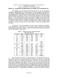
9 Produces the required equation. c Sd 2 DZ DR Re S0 =. 2 2. B l Page 3 of 41. Classic Transmission line Enclosure Alignment Tables By Martin J. King, 10/16/03 (revised 10/20/06). Copyright 2003 by Martin J. King. All Rights Reserved. If a value for DR is defined, the cross-sectional area at the closed end of the Transmission line can be calculated. table 3 contains recommended values for the resistance function for different values of driver Qts. Returning to the plot in Figure 6, the depth of the first null in the electrical impedance is being specified by calculating the value DR Re. For values of Qts outside of this range, extrapolation can be used to determine the appropriate value of the electrical impedance. The values of Qts contained in table 3 span most suitable drivers for Transmission line enclosures. Having calculated S0, and knowing SL/S0 and the effective length, the geometry of the Classic Transmission line Enclosure is completely defined. With this known geometry the only open issue is the driver location along the length of the Transmission line .

10 If the driver is mounted at the closed end of the Transmission line , then all of the higher harmonics of the fundamental quarter wavelength resonance will be excited. By offsetting the driver the excitation of certain higher modes can be reduced and even suppressed. table 4 contains the maximum recommended driver offset positions. At these driver positions, it is possible to almost completely suppress the second mode (three- quarter wavelength) and every other quarter wavelength mode (seven-quarter wavelength, eleven-quarter wavelength ) above this point. One consequence of offsetting the driver is a reduction in the excitation applied to the fundamental quarter wavelength mode, the tuning frequency of the line , and some reduction in bass extension. By placing the driver someplace between the closed end ( = 0) and the maximum offset ratio shown in table 4, a compromise response results. A commonly found recommendation for the driver offset ratio is Page 4 of 41.