Transcription of Answer to Mixed ANOVA Guided Example
1 C8057 (Research Methods II): Answer to Mixed ANOVA Guided Question Answer to Mixed ANOVA Guided Question What are the independent variables and how many levels do they have? The first IV is gender, which has two levels: Male and female. The second IV is type of drink', which has three levels: beer, wine and water. What is the dependent variable? The DV is the attitude towards the drink ( the rating on the scale ranging from -100. (dislike) to +100 (like). What analysis have you performed? ( and x by y what type of ANOVA ). A two-way 2 (gender: male or female) 3 (type of drink: beer, wine or water) Mixed ANOVA . with repeated measures on the type of drink variable.)
2 Has the assumption of sphericity been met? (Quote relevant statistics in APA. format). Mauchly's sphericity test for the repeated measures variable is shown below. The main effect of drink does not significantly violate the sphericity assumption because the significance value is greater than .05, W = .847, 2 (2) = , p > .05. Therefore, the F-value for the main effect of drink (and its interaction with the between-group variable gender) does not need to be corrected for violations of sphericity (see last handout). Mauchly's Test of Sphericityb Measure: MEASURE_1. a Mauchly's Approx. Epsilon Within Subjects Effect W Chi-Square df Sig.
3 Greenhouse-Geisser Huynh-Feldt Lower-bound DRINK .847 2 .243 .867 .500. Tests the null hypothesis that the error covariance matrix of the orthonormalized transformed dependent variables is proportional to an identity matrix. a. May be used to adjust the degrees of freedom for the averaged tests of significance. Corrected tests are displayed in the layers (by default) of the Tests of Within Subjects Effects table. b. Design: Intercept+GENDER. Within Subjects Design: DRINK. Report the main effect of type of drink in APA format. Is this effect significant and how would you interpret it? The summary table of the repeated measures effects in the ANOVA with corrected F-values is below.
4 The output is split into sections for each of the effects in the model and their associated error terms. The table format is the same as for other examples we have seen, except that the interactions between gender and the repeated-measures effects are included also. By looking at the significance values it is clear that there are significant effects of the type of drink used and the interaction of this and the gender of the participant. The fact that gender interacts significantly with the type of drink used tells us that men and women respond differently to the adverts for Beer, Wine and Water. Professor Andy Field, 2000 & 2003 Page 1.
5 C8057 (Research Methods II): Answer to Mixed ANOVA Guided Question Tests of Within-Subjects Effects Measure: MEASURE_1. Type III. Sum of Mean Source Squares df Square F Sig. DRINK Sphericity Assumed 2 .000. Greenhouse-Geisser .000. Huynh-Feldt .000. Lower-bound .000. DRINK * GENDER Sphericity Assumed 2 .000. Greenhouse-Geisser .000. Huynh-Feldt .000. Lower-bound .000. Error(DRINK) Sphericity Assumed 36 Greenhouse-Geisser Huynh-Feldt Lower-bound In APA format we could report: There was a significant main effect of drink, F(2, 36) = , p < .001. This effect tells us that if we ignore the gender of participants, some types of drink were still rated significantly differently to others.
6 If you requested that SPSS display means for all of the effects in the model (before conducting post hoc tests) and if you scan through your output you should find the table in a section headed Estimated Marginal Means. This is a table of means for the main effect of drink with the associated standard errors. The levels of this variable are labelled, 1, 2 and 3 and so we must think back to how we entered the variable to see which row of the table relates to which condition. We entered this variable with the beer condition first and the water condition last. The graph displays this information. It is clear from this graph that beer is naturally rated higher than wine and water (with beer being rated most highly).
7 To see the nature of this effect we can look at the post hoc tests (see below) and the contrasts (see section below). 5. Estimates 0. Measure: MEASURE_1 Beer Wine Water 95% Confidence Interval Lower Upper -5. DRINK Mean Std. Error Bound Bound 1 2 3 -10. -15 -12. The pairwise comparisons for the main effect of drink corrected using a Bonferroni adjustments are below. This table indicates that the significant main effect reflects a significant difference (p < .01) between levels 1 and 2 (beer and wine) and 1 and 3 (beer and water) but not between levels 2 and 3 (wine and water). This seems to indicate that negative imagery had an effect on ratings of both wine and water but not on beer.
8 Professor Andy Field, 2000 & 2003 Page 2. C8057 (Research Methods II): Answer to Mixed ANOVA Guided Question Pairwise Comparisons Measure: MEASURE_1. 95% Confidence Interval a Mean for Difference Difference Lower Upper a (I) DRINK (J) DRINK (I-J) Std. Error Sig. Bound Bound 1 2 * .000 3 * .000 2 1 * .000 3 .281 3 1 * .000 2 .281 Based on estimated marginal means *. The mean difference is significant at the .05 level. a. Adjustment for multiple comparisons: Bonferroni. Report the main effect of gender in APA format. Is this effect significant and how would you interpret it? The main effect of gender is listed separately from the repeated measure effects in a table labelled tests of between-subjects effects.
9 Before looking at this table it is important to check the assumption of homogeneity of variance using Levene's test (see Field, 2005 chapter 3 or your handout from week 2). SPSS produces a table listing Levene's test for each level of the repeated-measures variables in the Data Editor, and we need to look for any variable that has a significant value. The SPSS Output below shows both tables. The table showing Levene's test indicates that variances are homogenous for all levels of the repeated measures variables (because all significance values are greater than .05). The second table shows the ANOVA . summary table for the main effect of gender, and this reveals a significant effect (because the significance of , is less than the standard cut-off point of.)
10 05). a Levene's Test of Equality of Error Variances F df1 df2 Sig. Beer + Corpse 1 18 .268. Wine+ Corpse 1 18 .320. Water+ Corpse .804 1 18 .382. Tests the null hypothesis that the error variance of the dependent variable is equal across groups. a. Design: Intercept+GENDER. Within Subjects Design: DRINK. Tests of Between-Subjects Effects Measure: MEASURE_1. Transformed Variable: Average Type III. Sum of Mean Source Squares df Square F Sig. Intercept 1 .000. GENDER 1 .000. Error 18 In APA format we report that: There was a significant main effect of gender, F (1, 18) = , p < .001. This effect tells us that if we ignore all other variables, male participants' ratings were significantly different to females'.