Transcription of The t-test in IBM SPSS Statistics
1 Prof. Andy Field Page 1 The t-test in IBM spss Statistics An Example: are invisible people mischievous? In my spss book (Field, 2013) I imagine a future in which we have some cloaks of invisibility to test out. As a psychologist (with his own slightly mischievous streak) I might be interested in the effect that wearing a cloak of invisibility has on people s tendency for mischief. I took 24 participants and placed them in an enclosed community. The community was riddled with hidden cameras so that we could record mischievous acts. Half of them were given cloaks of invisibility: they were told not to tell anyone else about their cloak and that they could wear it whenever they liked. We measured how many mischievous acts they performed in a week. These data are in Table 1. The file shows how you should have entered the data: the variable Cloak records whether or not a person was given a cloak (cloak = 1) or not (cloak = 0), and Mischief is how many mischievous acts were performed.
2 Table 1: Data from Participant Cloak Mischief 1 0 3 2 0 1 3 0 5 4 0 4 5 0 6 6 0 4 7 0 6 8 0 2 9 0 0 10 0 5 11 0 4 12 0 5 13 1 4 14 1 3 15 1 6 16 1 6 17 1 8 18 1 5 19 1 5 20 1 4 21 1 2 22 1 5 23 1 7 24 1 5 Prof. Andy Field Page 2 The independent t-test using spss The general procedure Figure 1 shows the general process for performing a t-test : as with fitting any model, we start by looking for the sources of bias. Having satisfied ourselves that assumptions are met and outliers dealt with, we run the test. We can also consider using bootstrapping if any of the test assumptions were not met. Finally, we compute an effect size. Figure 1: The general process for performing a t-test Compute the independent t-test To run an independent t-test , we need to access the main dialog box by selecting (see Figure 2). Once the dialog box is activated, select the dependent variable from the list (click on Mischief) and transfer it to the box labelled Test Variable(s) by dragging it or clicking on.
3 If you want to carry out t- tests on several dependent variables then you can select other dependent variables and transfer them to the variables list. However, there are good reasons why it is not a good idea to carry out lots of tests . Next, we need to select an independent variable (the grouping variable). In this case, we need to select Cloak and then transfer it to the box labelled Grouping Variable. When your grouping variable has been selected the button will become active and you should click on it to activate the Define Groups dialog box. spss needs to know what numeric codes you assigned to your two groups, and there is a space for you to type the codes. In this example, we coded our no cloak group as 0 and our cloak group as 1, and so these are the codes that we type. When you have defined the groups, click on to return to the main dialog box.
4 If you click on then another dialog box appears that gives you the chance to change the width of the confidence interval that is calculated. The default setting is for a 95% confidence interval and this is fine; however, if you want to be stricter about your analysis you could choose a 99% confidence interval but you run a higher risk of failing to detect a genuine effect (a Type II error). To run the analysis click on . If we have potential bias in the data we can reduce its impact by using bootstrapping to generate confidence intervals for the difference between means. We can select this option by clicking in the main dialog box to access the bootstrap function. Select to activate bootstrapping, and to get a 95% confidence interval click or Calculate an effect sizeBoxplots, histograms, descriptive statisticsRun the t-testBootstrap if problems with the dataExplore dataCheck for outliers, normality, homogeneity etc.
5 Prof. Andy Field Page 3 . For this analysis, let s ask for a bias corrected (BCa) confidence interval. Back in the main dialog box click on to run the analysis. Figure 2: Dialog boxes for the independent-samples t-test Output from the independent t-test (1) The output from the independent t-test contains only three tables (two if you don t opt for bootstrapping). The first table (Output 1) provides summary Statistics for the two experimental conditions (if you don t ask for bootstrapping this table will be a bit more straightforward). From this table, we can see that both groups had 12 participants (row labelled N). The group who had no cloak, on average, performed mischievous acts with a standard deviation of What s more, the standard error of that group is The bootstrap SE estimate is .53, and the bootstrapped confidence interval for the mean ranges from to For those that were given an invisibility cloak, they performed, on average, 5 acts, with a standard deviation of , a standard error of The bootstrap standard error is a bit lower at , and the confidence interval for the mean ranges from to Note that the confidence intervals for the two groups overlap, implying that they might be from the same population.
6 The second table of output (Output 2) contains the main test Statistics . The first thing to notice is that there are two rows containing values for the test Statistics : one row is labelled Equal variances assumed, while the other is labelled Equal variances not assumed. Parametric tests assume that the variances in experimental groups are roughly equal. The rows of the table relate to whether or not this assumption has been broken. Prof. Andy Field Page 4 Output 1 We can use Levene s test to see whether variances are different in different groups (although there are problems with this test discussed in my book), and spss produces this test for us. Levene s test tests the hypothesis that the variances in the two groups are equal. Therefore, if Levene s test is significant at p .05, it suggests that the assumption of homogeneity of variances has been violated.
7 If, however, Levene s test is non-significant ( , p > .05) then we can assume that the variances are roughly equal and the assumption is tenable. For these data, Levene s test is non-significant (because p = .468, which is greater than .05) and so we should read the test Statistics in the row labelled Equal variances assumed. Had Levene s test been significant, then we would have read the test Statistics from the row labelled Equal variances not assumed. Output 2 Having established that the assumption of homogeneity of variances is met, we can look at the t-test itself. We are told the mean difference ( "# # = 5 = ) and the standard error of the sampling distribution of differences. The t-statistic is , which is assessed against the value of t you might expect to get if there was no effect in the population when you have certain degrees of freedom.
8 For the independent t-test , degrees of freedom are calculated by adding the two sample sizes and then subtracting the number of samples (df = N1 + N2 2 = 12 + 12 2 = 22). spss produces the exact significance value of t, and typically we are interested in whether this value is less than or greater than .05. In this case the two-tailed value of p is .107, which is greater than .05, and so we would have to conclude that there was no significant difference between the means of these two samples. In terms of the experiment, we can infer that having a cloak of invisibility did not significantly affect the amount of mischief a person got up to. Output 3 Prof. Andy Field Page 5 Output 3 shows the results of the bootstrapping (if you selected it). You can see that the bootstrapping procedure has been applied to re-estimate the standard error of the mean difference (which is estimated as.)
9 726 rather than .730). Using this bootstrapped standard error confidence intervals for the difference between means are computed. The difference between means was , and the confidence interval ranged from to The confidence interval implies that the difference between means in the population could be negative, positive or even zero (because the interval ranges from a negative value to a positive one). In other words, it s possible that the true difference between means is zero no difference at all. Therefore, this bootstrap confidence interval confirms our conclusion that having a cloak of invisibility seems not to affect acts of mischief. Reporting the independent t-test (1) You usually state the finding to which the test relates and then report the test statistic, its degrees of freedom and the probability value of that test statistic.
10 We could write: On average, participants given a cloak of invisibility engaged in more acts of mischief (M = 5, SE = ), than those not given a cloak (M = , SE = ). This difference, , BCa 95% CI [ , ], was not significant t(22) = , p = .101; however, it did represent a medium-sized effect d = .65. Matched-samples t-test using spss Entering Data Let s imagine that we had collected the cloak of invisibility data using a repeated measures design; so, the data are identical to before. In this scenario we might have recorded everyone s natural level of mischievous acts in a week, then given them an invisibility cloak and counted the number of mischievous acts in the next week. The data would now be arranged differently in spss . Instead of having a coding variable, and a single column with mischief scores in, we would arrange the data in two columns (one representing the Cloak condition and one representing the No_Cloak condition).