Transcription of Blind Source Separation: PCA & ICA - mit.edu
1 D. Clifford gari [at] mit . ~gari G. D. Clifford 2005-2009 Blind Source Separation: PCA & ICAWhat is BSS?Assume an observation (signal) is a linear mix of >1 unknown independentsource signalsThe mixing (not the signals) is stationaryWe have as manyobservations as unknown sources To find sources in observations- need to define a suitable measure of For example - the cocktail party problem(sources are speakers and background noise):The cocktail party problem - find ZAz1z2zNXTZTXT=AZTx1x2xN2 Formal statement of problem N independentsources ..Zmn( MxN) linear square mixing ..Ann( NxN) (#sources=#sensors) produces a set of observations ..Xmn( MxN).. XT= AZTF ormal statement of solution demix observations ..XT( NxM)into YT= WXTYT(NxM) ZTW(NxN) A-1 How do we recover the independent sources? (We are trying to estimate W A-1).. We require a measure of independence! Signal Source Noise sourcesObserved mixturesZTXT=AZTYT=WXT3XT = A ZTYT = W XTTTTTThe Fourier Transform(Independence between components is assumed) Recap: Non-causal Wiener filteringx[n] - observationy[n] - ideal signald[n] - noise componentIdeal Signal Sy(f)Noise Power Sd(f)Observation Sx(f)Filtered signal: Sfilt(f ) = Sx(f).
2 H(f )f4 BSS is a transform? Like Fourier, we decompose into components by transforming the observations into another vector space which maximises the separationbetween interesting (signal) and unwanted (noise). Unlike Fourier, separation is not based on frequency-It s based on independence Sources can have the same frequency content No assumptionsabout the signals (other than they are independentand linearlymixed) So you can filter/separate in-bandnoise/signals with BSSP rincipal Component Analysis Second orderdecorrelation= independence Find a set of orthogonalaxes in the data (independence metric = variance) Project data onto these axes to decorrelate Independenceis forced onto the data through the orthogonalityof axes Conventional noise / signal separation techniqueSingular Value DecompositionDecompose observation X= X=USVT Sis a diagonal matrix of singular values with elements arranged in descending order of magnitude (the singular spectrum) The columns of Vare the eigenvectors of C=XTX(the orthogonal subspace.)
3 Dot(vi,vj)=0 ) .. they demix or rotate the data Uis the matrix of projections of Xonto the eigenvectors of C ..the Source estimates5 Singular Value DecompositionDecompose observation X= X=USVTE igenspectrum of decomposition S= singularmatrix .. zeros except on the leading diagonal Sij(i=j) are the eigenvalues Placed in order of descending magnitude Correspond to the magnitude of projected data along each eigenvector Eigenvectors are the axes of maximal variation in the dataVariance = power (analogous to Fourier components in power spectra)[stem(diag(S).^2)]Eigenspectrum= Plot of eigenvaluesSVD: Method for PCA6 SVD noise/signal separationTo perform SVD filtering of a signal, use a truncated SVD decomposition (using the first peigenvectors)Y=USpVT[Reduce the dimensionality of the data by discarding noise projections Snoise=0 Then reconstruct the data with just the signal subsapce] Most of the signal is contained in the first few principal these and projecting back into the original observation space effects a noise-filtering or a noise/signal separationReal dataXXp= dimensional example7 IndependentComponent AnalysisAs in PCA, we are looking for Ndifferent vectors onto which we can project our observations to give a set of N maximally independent signals(sources) output data (discovered sources) dimensionality = dimensionality of observations Instead of using varianceas our independence measure ( decorrelating) as we do in PCA, we use a measure of how statistically independentthe sources : The basic idea.
4 Assume underlying Source signals (Z) are a linear mixing matrix (A)..XT=AZTin order to find Y( Z), find W, ( A-1) ..YT=WXTHow?Initialise W& iteratively update Wto minimise or maximise a cost function that measures the (statistical) independencebetween the columns of the statistical independence?From the Central Limit Theorem, - add enough independent signals together, Gaussian PDF Sources,ZP(Z) (subGaussian)Mixtures (XT=AZT)P(X) (Gaussian) Recap: Moments of a distribution9 Higher order moments (3rd -skewness) xHigher order moments (4th-kurtosis) xSuperGaussianSubGaussianGaussians are mesokurticwith =3 Non-Gaussianity statistical independence?Central Limit Theorem: add enough independent signals together, Gaussian PDF make data components non-Gaussian to find independent sourcesSources,ZP(Z) ( <3 ( ) )Mixtures (XT=AZT)P(X) ( = ) ( =3)10 Recall trying to estimate WAssume underlying Source signals (Z) are a linear mixing matrix (A).
5 XT=AZTin order to find Y( Z), find W, ( A-1) ..YT=WXTI nitialise W& iteratively update Wwith gradient descent to maximise descent to find W Given a cost function, , we update each element of W ( ) at each step, , .. and recalculate cost function ( is the learning rate (~ ), and speeds up convergence.)wijW=[1 3; -2 -1]Iterationswij 105 Weight updates to find:(Gradient ascent)11 Gradient descentmin (1/| 1|, 1/| 2|) | = maxGradient Descent = min (1/| 1|, 1/| 2|) | = max Cost function, , can be maximum or minimum 1/ Gradient descent example Imagine a 2-channel ECG, comprised of two sources; Cardiac and SNR=1 X1X212 Iteratively update W and measure Y1Y2 Iteratively update W and measure Y1Y2 Iteratively update W and measure Y1Y214 Iteratively update W and measure Y1Y2 Iteratively update W and measure Y1Y2 Maximized for non-Gaussian signalY1Y215 Outlier insensitive ICA cost functionsIn general we require a measure of statistical independence which we maximise betweeneach of the is one approximation, but sensitive to small changes in the distribution tail.
6 Other measures include:Measures of statistical independence Mutual Information II, Entropy (Negentropy, JJ).. and Maximum (Log) Likelihood (Note: all are related to )Entropy-based cost functionKurtosis is highly sensitive to small changes in distribution tails. A more robust measures of Gaussianity is based on differential entropy H(y), ..negentropy:where ygaussis a Gaussian variable with the same covariance matrix as y. J(y) can be estimated from kurtosis ..Entropy: measure of randomness- Gaussians are maximally random16 Minimising Mutual InformationMutual information (MI) between two vectors xand y :always non-negative and zero if variables are independent ..therefore we want to minimise can be re-written in terms of negentropy ..where cis a constant.. differs from negentropy by a constant and a sign changeII= Hx+ Hy-HxyGenerative latent variable modelling Nobservables, from Nsources, zithrough a linear mapping W=wijLatent variables assumed to be independently distributedFind elements of W by gradient ascent - iterative update bywhere is some learning rate (const).
7 Andis our objective cost function, the log likelihoodIndependent Source discovery using Maximum some real examples using ICAThe cocktail party problem revisited1718 Why? .. In XT=AZT, insert a permutation matrix B ..XT=ABB-1ZT = sources with different col. order. sources change by a scaling ICA solutions are order and scale independent because is dimensionlessObservationsSeparation of mixed observations into Source estimates is excellent .. apart from: Order of sources has changed Signals have been scaledSeparation of sources in the ECG =3 =11 =0 =3 =1 =5 =0 = 19 Transformation inversion for filtering Problem - can never know if sources are really reflective of the actual Source generators - no gold standard De-mixing might alter the clinical relevance of the ECG features Solution: Identify unwanted sources, set corresponding (p) columns in W-1to zero (Wp-1), then multiply back through to remove noise sources and transform back into original observation inversion for filteringReal dataXY=WX ZXfilt=Wp-1Y20 ICA results 4XY=WX ZXfilt=Wp-1Y PCA is good for Gaussian noise separation ICA is good for non-Gaussian noise separation PCs have obvious meaning - highest energy components ICA - derived sources.
8 Arbitrary scaling/inversion & need energy-independent heuristic to identify signals / noise Order of ICs change - IC space is derivedfrom the data. - PC space only changes if SNR changes. ICA assumes linear mixing matrix ICA assumesstationarymixing De-mixing performance is function of lead position ICA requires as manysensors (ECG leads) as sources Filtering - discard certain dimensions then invert transformation In-band noise can be removed - unlike Fourier!SummaryFetal ECG lab preparation21 Fetal abdominal recordings Maternal ECG is much larger in amplitude Maternal and fetal ECG overlap in time domain Maternal features are broader, but Fetal ECG is in-bandof maternal ECG (they overlap in freq domain) 5 second window .. Maternal HR=72 bpm / Fetal HR = 156bpmMaternal QRSF etal QRSMECG & FECG spectral propertiesFetal QRS power regionECG EnvelopeMovement ArtifactQRS ComplexP & T WavesMuscle NoiseBaseline WanderFetal /Maternal MixtureMaternalNoise Fetal