Transcription of Bode Plot: Example 1 - utoledo.edu
1 Bode Plot: Example 1 Draw the Bode Diagram for the transfer function: Step 1: Rewrite the transfer function in proper form. Make both the lowest order term in the numerator and denominator unity. The numerator is an order 0 polynomial, the denominator is order 1. Step 2: Separate the transfer function into its constituent parts. The transfer function has 2 components: A constant of A pole at s=-30 Step 3: Draw the Bode diagram for each part. This is done in the diagram below. The constant is the cyan line (A quantity of is equal to dB). The phase is constant at 0 degrees. The pole at 30 rad/sec is the blue line. It is 0 dB up to the break frequency, then drops off with a slope of -20 dB/dec. The phase is 0 degrees up to 1/10 the break frequency (3 rad/sec) then drops linearly down to -90 degrees at 10 times the break frequency (300 rad/sec). Step 4: Draw the overall Bode diagram by adding up the results from step 3. The overall asymptotic plot is the translucent pink line, the exact response is the black line.
2 Bode Plot: Example 2 Draw the Bode Diagram for the transfer function: Step 1: Rewrite the transfer function in proper form. Make both the lowest order term in the numerator and denominator unity. The numerator is an order 1 polynomial, the denominator is order 2. Step 2: Separate the transfer function into its constituent parts. The transfer function has 4 components: A constant of A pole at s=-10 A pole at s=-100 A zero at s=-1 Step 3: Draw the Bode diagram for each part. This is done in the diagram below. The constant is the cyan line (A quantity of is equal to -20 dB). The phase is constant at 0 degrees. The pole at 10 rad/sec is the green line. It is 0 dB up to the break frequency, then drops off with a slope of -20 dB/dec. The phase is 0 degrees up to 1/10 the break frequency (1 rad/sec) then drops linearly down to -90 degrees at 10 times the break frequency (100 rad/sec). The pole at 100 rad/sec is the blue line. It is 0 dB up to the break frequency, then drops off with a slope of -20 dB/dec.
3 The phase is 0 degrees up to 1/10 the break frequency (10 rad/sec) then drops linearly down to -90 degrees at 10 times the break frequency (1000 rad/sec). The zero at 1 rad/sec is the red line. It is 0 dB up to the break frequency, then rises at 20 dB/dec. The phase is 0 degrees up to 1/10 the break frequency ( rad/sec) then rises linearly to 90 degrees at 10 times the break frequency (10 rad/sec). Step 4: Draw the overall Bode diagram by adding up the results from step 3. The overall asymptotic plot is the translucent pink line, the exact response is the black line. Bode Plot: Example 3 Draw the Bode Diagram for the transfer function: Step 1: Rewrite the transfer function in proper form. Make both the lowest order term in the numerator and denominator unity. The numerator is an order 1 polynomial, the denominator is order 2. Step 2: Separate the transfer function into its constituent parts. The transfer function has 4 components: A constant of A pole at s=-3 A pole at s=0 A zero at s=-10 Step 3: Draw the Bode diagram for each part.
4 This is done in the diagram below. The constant is the cyan line (A quantity of is equal to 30 dB). The phase is constant at 0 degrees. The pole at 3 rad/sec is the green line. It is 0 dB up to the break frequency, then drops off with a slope of -20 dB/dec. The phase is 0 degrees up to 1/10 the break frequency ( rad/sec) then drops linearly down to -90 degrees at 10 times the break frequency (30 rad/sec). The pole at the origin. It is a straight line with a slope of -20 dB/dec. It goes through 0 dB at 1 rad/sec. The phase is -90 degrees. The zero at 10 rad/sec is the red line. It is 0 dB up to the break frequency, then rises at 20 dB/dec. The phase is 0 degrees up to 1/10 the break frequency (1 rad/sec) then rises linearly to 90 degrees at 10 times the break frequency (100 rad/sec). Step 4: Draw the overall Bode diagram by adding up the results from step 3. The overall asymptotic plot is the translucent pink line, the exact response is the black line.
5 Bode Plot: Example 4 Draw the Bode Diagram for the transfer function: Step 1: Rewrite the transfer function in proper form. Make both the lowest order term in the numerator and denominator unity. The numerator is an order 1 polynomial, the denominator is order 3. Step 2: Separate the transfer function into its constituent parts. The transfer function has 4 components: A constant of -10 A pole at s=-10 A doubly repeated pole at s=-1 A zero at the origin Step 3: Draw the Bode diagram for each part. This is done in the diagram below. The constant is the cyan line (A quantity of 10 is equal to 20 dB). The phase is constant at -180 degrees (constant is negative). The pole at 10 rad/sec is the blue line. It is 0 dB up to the break frequency, then drops off with a slope of -20 dB/dec. The phase is 0 degrees up to 1/10 the break frequency then drops linearly down to -90 degrees at 10 times the break frequency. The repeated pole at 1 rad/sec is the green line.
6 It is 0 dB up to the break frequency, then drops off with a slope of -40 dB/dec. The phase is 0 degrees up to 1/10 the break frequency then drops linearly down to -180 degrees at 10 times the break frequency. The magnitude and phase drop twice as steeply as those for a single pole. The zero at the origin is the red line. It has a slope of +20 dB/dec and goes through 0 dB at 1 rad/sec. The phase is 90 degrees. Step 4: Draw the overall Bode diagram by adding up the results from step 3. The overall asymptotic plot is the translucent pink line, the exact response is the black line. Bode Plot: Example 5 Draw the Bode Diagram for the transfer function: Step 1: Rewrite the transfer function in proper form. Make both the lowest order term in the numerator and denominator unity. The numerator is an order 1 polynomial, the denominator is order 2. Step 2: Separate the transfer function into its constituent parts. The transfer function has 4 components: A constant of 6 A zero at s=-10 Complex conjugate poles at the roots of s2+3s+50, with Step 3: Draw the Bode diagram for each part.
7 This is done in the diagram below. The constant is the cyan line (A quantity of 6 is equal to dB). The phase is constant at 0 degrees. The zero at 10 rad/sec is the green line. It is 0 dB up to the break frequency, then rises with a slope of +20 dB/dec. The phase is 0 degrees up to 1/10 the break frequency then rises linearly to +90 degrees at 10 times the break frequency. The plots for the complex conjugate poles are shown in blue. They cause a peak of: at a frequency of This is shown by the blue circle. The phase goes from the low frequency asymptote (0 degrees) at to the high frequency asymptote at Step 4: Draw the overall Bode diagram by adding up the results from step 3. The exact response is the black line. Bode Plot: Example 6 Draw the Bode Diagram for the transfer function: Step 1: Rewrite the transfer function in proper form. Make both the lowest order term in the numerator and denominator unity.
8 The numerator is an order 2 polynomial, the denominator is order 3. Step 2: Separate the transfer function into its constituent parts. The transfer function has 4 components: A constant of 1 A pole at s=-100 A repeated pole at the origin (s=0) Complex conjugate zeros at the roots of s2+s+25, with Step 3: Draw the Bode diagram for each part. This is done in the diagram below. The constant is the cyan line (A quantity of 1 is equal to 0 dB). The phase is constant at 0 degrees. The pole at 100 rad/sec is the green line. It is 0 dB up to the break frequency, then falls with a slope of -20 dB/dec. The phase is 0 degrees up to 1/10 the break frequency then falls linearly to -90 degrees at 10 times the break frequency. The repeated poles at the origin are shown with the blue line. The slope is -40 dB/decade (because pole is repeated), and goes through 0 dB at 1 rad/sec. The slope is -180 degrees (again because of double pole). The complex zero is shown by the red line.
9 The zeros give a dip in the magnitude plot of at a frequency of 5 rad/sec (because is small, r 0). This is shown by the red circle. The phase goes from the low frequency asymptote (0 degrees) at to the high frequency asymptote at Again, because is so small, this line is close to vertical. Step 4: Draw the overall Bode diagram by adding up the results from step 3. The exact response is the black line. Bode Plot: Example 7 Draw the Bode Diagram for the transfer function: This is the same as " Example 1," but has a second time delay. We have not seen a time delay before this, but we can easily handle it as we would any other constituent part of the transfer function. The magnitude and phase of a time delay are described here. Step 1: Rewrite the transfer function in proper form. Make both the lowest order term in the numerator and denominator unity. The numerator is an order 0 polynomial, the denominator is order 1.
10 Step 2: Separate the transfer function into its constituent parts. The transfer function has 3 components: A constant of A pole at s=-30 A time delay of seconds (magnitude and phase of time delay described here). Step 3: Draw the Bode diagram for each part. This is done in the diagram below. The constant is the cyan line (A quantity of is equal to dB). The phase is constant at 0 degrees. The pole at 30 rad/sec is the blue line. It is 0 dB up to the break frequency, then drops off with a slope of -20 dB/dec. The phase is 0 degrees up to 1/10 the break frequency (3 rad/sec) then drops linearly down to -90 degrees at 10 times the break frequency (300 rad/sec). The time delay is the red line. It is 0 dB at all frequencies. The phase of the time delayis given by rad, or 180/ (at =100 rad/sec, the phase is 100 180/ -30 ). There is no asymptotic approximation for the phase of a time delay. Though the equation for the phase is linear with frequency, it looks exponential on the graph because the horizontal axis is logarithmic.
![CHAP. 7] BLOCK DIAGRAM ALGEBRA AND TRANSFER …](/cache/preview/5/5/8/8/1/3/4/c/thumb-5588134cce7b9b85f7cd5a0611a184e9.jpg)