Transcription of Bode plots
1 Engineering Sciences 22 Systems Summer 2004. BODE plots . A Bode plot is a standard format for plotting frequency response of LTI systems. Becoming familiar with this format is useful because: 1. It is a standard format, so using that format facilitates communication between engineers. 2. Many common system behaviors produce simple shapes ( straight lines) on a Bode plot , so it is easy to either look at a plot and recognize the system behavior, or to sketch a plot from what you know about the system behavior. The format is a log frequency scale on the horizontal axis and, on the vertical axis, phase in degrees and magnitude in decibels. Thus, we begin with a review of decibels 1. Decibels Definition: for voltages or other physical variables (current, velocity, pressure, etc.). Vout decibels (dB) = 20 log10 V , in (Since power is propotional to voltage squared (or current, velocity, pressure, etc., squared) the definition can be rewritten in terms of power as Vout Vout 2 Pout decibels (dB) = 20 log10 V = 10 log10 V = 10 log10 P.)
2 In in in Common values 10 log10 2 = 20 log10 2 = 3 dB. 1 1. 10 log10 2 = 20 log10 = 3 dB half power . 2. 10 log10 10 = 20 log10 10 = 10 dB. 10 log10 100 = 20 log10 10 = 20 dB, etc 10 dB for every factor of 10 in power 2. Bode plots We are interested in the frequency response of an LTI system. The transfer function can be written like this: ( s z1 )( s z 2 ) L. H (s) = K. ( s p1 )( s p 2 )( s p3 ) L. such that when we plug in j for s, we get ( j z1 )( j z 2 ) L. H ( j ) = K. ( j p1 )( j p 2 )( j p3 ) L. Bode plots Page 1. Engineering Sciences 22 Systems Summer 2004. That's a product (or quotient) of a bunch of complex numbers. Using polar form, we can say that the angle of the product (quotient) is the sum of the angles of each term (except for division we subtract, so it's the sum of the angles for the top terms, minus the sum of the angles for the terms in the denominator). Similarly, the magnitude is the product of the magnitude of all the terms. Summing terms is easy to do graphically; products are harder.
3 However, on a log scale ( , dB), the product turns into a sum. Thus, if we plot the behavior of each term, we can then simply add the plots to find the total behavior. For the poles, we could either plot the behavior of (s - p) and subtract it, or plot the behavior of 1/(s - p) and add that behavior. We'll plot the behavior of 1/(s - p), such that we only need to add terms. The general plan for how to sketch a Bode plot by hand is, then, to first gain an understanding of what individual poles and individual zeros do, and then add the responses together. It is easiest to understand complex poles and zeros by looking at the response of a complex conjugate pair, rather than trying to look at the complex poles or zeros individually. This handout includes some information on complex pairs, but you aren't required to learn how to sketch a Bode plot with them for ENGS 22. The following pages contain, first, a catalog of responses you can expect from individual poles and zeros, and then step-by-step instructions on how to construct a Bode plot from a transfer function.
4 The examples given on the following pages all have a normalized (unitless) frequency scale, in /a where a is the pole or zero, and = 2 f, rather than the usual frequency scale in Hz. The idea is that the point labeled 1 on the plot will appear at the frequency corresponding to the pole or zero (f = a/(2 )) on the real Bode plot you construct. Bode plots Page 2. Engineering Sciences 22 Systems Summer 2004. 2. Asymptotic properties of the frequency response a Single pole, H(s) = s + a 0. -10. Magnitude (dB). -20. -30. -40. 10 -2 10 -1 10 0 10 1 10 2. 0. Phase (deg). -45. -90 -2. 10 10 -1 10 0 10 1 10 2. w/a Magnitude response Low- frequency asymptote ( 0), flat Breakpoint at = a High frequency asymptote, 20 dB/decade Actual curve is 3 dB below breakpoint Phase response Low frequency asymptote = 0 . 45 at breakpoint ( = a). High frequency asymptote = 90 . Not required for ENGS 22: Central slope crosses 0 at a/5, 90 at 5a (if you care about doing it that accurately, it might be time to plot it with MATLAB).
5 Bode plots Page 3. Engineering Sciences 22 Systems Summer 2004. Single zero, H(s) = (s + b)/b 40. 30. Magnitude (dB). 20. 10. 0. 10 -2 10 -1 10 0 10 1 10 2. 90. Phase (deg). 45. 0 -2. 10 10 -1 10 0 10 1 10 2. w/b Magnitude response Low- frequency asymptote ( 0), flat Breakpoint at = b High frequency asymptote, +20 dB/decade Actual curve is +3 dB above breakpoint Phase response Low frequency asymptote = 0 . +45 at breakpoint ( = b). High frequency asymptote = +90 . Not required for ENGS 22: Central slope crosses 0 at b/5 +90 at 5b Bode plots Page 4. Engineering Sciences 22 Systems Summer 2004. a2. Double pole, H(s) =. (s+a)2. You could derive this result from two individual poles it's just the sum of two of them. 0. -20. Magnitude (dB). -40. -60. -80. -100 -2 -1 0 1 2. 10 10 10 10 10. 0. Phase (deg). -90. -180 -2. 10 10 -1 10 0 10 1 10 2. w/a Magnitude response Low- frequency asymptote ( 0), flat Breakpoint at = a High frequency asymptote, 40 dB/decade Actual curve is 6 dB below breakpoint Phase response Low frequency asymptote = 0.
6 90 at breakpoint ( = a). High frequency asymptote = 180 . Not required for ENGS 22: Central slope crosses 0 at a/5, 180 at 5a Bode plots Page 5. Engineering Sciences 22 Systems Summer 2004. 3. Second order underdamped response (for reference only not required knowledge for 22). n2. Two poles, underdamped, H(s) = 2. s + 2 n s + n2. 20 log10|H(j )| H(j ). Exact = n 1. 20 log10 dB 90 . 2 . << n 0 dB 0 . >> n 40 dB/decade 180 . 20. = = Gain (dB). 0. = -20. -40. -1 0 1. 10 10 10. 0. Phase (degrees). -45. -90. -135. -180. -1 0 1. 10 10 10. Normalized frequency / n Bode plots Page 6. Engineering Sciences 22 Systems Summer 2004. (second-order underdamped, continued). Magnitude response Low- frequency asymptote ( 0), flat Breakpoint at = n High frequency asymptote, 40 dB/decade Resonant peak is at height 1/(2 ). The actual maximum occurs at = n 1 2 2 , and the actual maximum value is 1.. For sufficiently small , this point coincides with n and 1/(2 ). 2 1 2. Phase response Low frequency asymptote = 0.
7 90 at breakpoint ( = a). High frequency asymptote = 180 . Central slope crosses 0 at n/5 , 180 at 5 n ns Other second order responses: H(s) = 2 and s + 2 n s + n2. s2. H(s) = 2 (bandpass and highpass, respectively) ; the asymptotes are s + 2 n s + n2. different, but they always cross at 0 dB, and the slope change from low to high is always 40. dB/decade. Quality factor (Q). n Empirical definition: For a resonant peak, Q = , = distance between half- . power ( 3dB) points. With this, the height of a resonant peak is Q and and bandwidth is n/Q . energy stored General definition: Q = 2 at resonance. energy lost per cycle Relationship to damping factor: Q = 1/2 . Bode plots Page 7. Engineering Sciences 22 Systems Summer 2004. 4. Hand Sketching: Step-by-step approach Put transfer function in ZPK form (factored zeros and poles, with a constant multiplier K out front). Identify breakpoints: distance of poles and zeros from the origin. Mark those on the frequency axis of the plot . Remember to convert from rad/sec to Hz.
8 Determine low or high frequency constant asymptote of gain by taking the limit of H(s) as s 0 or infinity, respectively. Convert to dB. Start at one of the asymptotes that is constant. (see below if neither is constant). Move along in frequency until you get to a breakpoint. Each breakpoint is associated with a change in slope of +/-20 dB/decade (+/-6 dB/octave). From left to right, a zero produces an increase in slope (The increase could be from negative to less negative, or from positive to more positive, etc.) Each pole produces a decrease in slope. Work through all the breakpoints, and check that the final asymptote is correct. Sketch in a smoother curve, 3 dB below or above each breakpoint (unless it is a double pole or zero in which case it is 6 dB below or above). Now fill in the phase by the same procedure: Find the phase on the asymptotes by looking at the limit of H(j ) as 0 or infinity. If the limit is real, the phase is 180 degrees or zero. If the limit is imaginary, the phase is +/-90 degress (-90 for a negative imaginary limit).
9 If the limit is zero, you have to look at what direction it came in to zero from. If it came from a positive imaginary number, the phase is 90 degree; a negative imaginary number -90. degrees. If it came from a positive real number, the phase is 0, and if it came from a negative real number, the phase is -90 Then from left to right, each pole causes a 90 transition in phase, and every zero causes a +90 transition in phase. You can use the rules for the slope of the transition, but it's usually not worth the trouble to get that exact. OK, what if neither asymptote is flat? For example H(s) = s/[(s+1)(s+100)]: HF limit: s/100 -> 0. LF limit: s/(s2) -> 0. Solution: Consider the shape it will look like: with breakpoints at 1/(2 ) and 100/(2 ). Instead of starting at HF or LF asymptotes, you can start with the flat center part. Consider the approximate value there, where s>>1 and s<<100. Then we can write the transfer function, putting the negligible stuff in a small font: H(s) = s/[(s+1)(s+100)] Then.
10 Thus, we can approximate H(s) as s/[100s] = 1/100 or 40 dB in the flat middle part. Then we can start there and sketch the rest. (It slopes down with +/- 20 dB/decade slope on either side of the plateau.). Bode plots Page 8.