Transcription of Chapter 11 Density of States, Fermi Energy and Energy Bands
1 11-1 Chapter 11 Density of states , Fermi Energy and Energy Bands Contents Chapter 11 Density of states , Fermi Energy and Energy Bands .. 11-1 Contents .. 11-1 Current and Energy Transport .. 11-1 Electron Density of states .. 11-2 Dispersion Relation .. 11-2 Effective Mass .. 11-3 Density of states .. 11-5 Fermi -Dirac Distribution .. 11-7 Electron Concentration .. 11-8 Fermi Energy in Metals .. 11-9 EXAMPLE Fermi Energy in Gold .. 11-11 Fermi Energy in Semiconductors .. 11-12 EXAMPLE Fermi Energy in Doped Semiconductors .. 11-13 Energy Bands .. 11-14 Multiple Bands .. 11-15 Direct and Indirect 11-16 Periodic Potential (Kronig-Penney Model) .. 11-17 Problems .. 11-24 References .. 11-24 Current and Energy Transport The electric field E is interfered with two processes which are the electric current Density j and the temperature gradientT.
2 The coefficients come from the Ohm s law and the Seebeck effect. The field can be written as 11-2 Tj ( ) where is the electrical conductivity and is the Seebeck coefficient. The heat flux (thermal current Density ) qis also interfered with both the electric field and the temperature gradientT . However, the coefficients are not readily attainable. Thomson in 1854 arrived at the relationship assuming that thermoelectric phenomena and thermal conduction are independent. Later, Onsager [1] supported that relationship by presenting the reciprocal principle which was experimentally verified. The heat flux can be written as TkTjq ( ) where k is the thermal conductivity consisting of the electronic and lattice (or phonon) contributions to the thermal conductivity as lekkk ( ) In this Chapter , only the electronic contribution to the total thermal conductivity is used.
3 TkTjqee ( ) We consider a one-dimensional analysis in this Chapter because most thermoelectric devices reasonably holds one-dimension, so that tensor notations are avoided. Electron Density of states Dispersion Relation From Equation ( ) (combining the Bohr model and the de Broglie wave), we have ph ( ) This is known as the de Broglie wavelength. Using the definition of wavevector k = 2 / , we have 11-3 pk ( ) Knowing the momentum p = mv, the possible Energy states of a free electron is obtained mkmpmvE22212222 ( ) which is called the dispersion relation ( Energy or frequency-wavevector relation). Effective Mass In reality, an electron in a crystal experiences complex forces from the ionized atoms. We imagine that the atoms in the linear chain form the electrical periodic potential.
4 If the free electron mass m is replaced by the effective mass m*, we can treat the motion of electrons in the conduction band as free electrons. An exact defined value of the wavevector k, however, implies complete uncertainty about the electron s position in real space. Mathematically, localization can be described by expressing the state of the electron as a wave packet, in other words, a group velocity. The group velocity of electrons in Figure is the slope of the dispersion relation. kvg ( ) Since the wavelength is twice the lattice constant a, the boundaries at the zone in k-space is k = /a. The frequency associated with a wavevector of Energy E is Eand pk ( ) where the two equations are known as the Planck-Einstein relations. 11-4 Figure Dispersion relation of a group of electrons with a nearest neighbor interaction.
5 Note that is linear for small k, and that k vanishes at the boundaries of the Brillouin zone (k = /a) kEvg 1 ( ) The derivative of Equation ( ) with respect to time is tkkEtkEtvg 22211 ( ) From Equation ( ), we have kmvg and tktvmg . The force acting on the group of electrons is then tktvmFg ( ) Combining Equations ( ) and ( ) yields tvkEFg 222 ( ) This indicates that there is an effective mass m*, which will replace the electron mass m. 22211kEm ( ) 11-5 The effective mass m* is the second order of derivative of Energy with respect to wavevector, which is representative of the local curvature of the dispersion relation in three dimensional space. The effective mass is a tensor and may be obtained experimentally or numerically. Density of states Thermoelectric materials typically exhibit the directional behavior.
6 Therefore, in general we have zzyyxxmkmkmkE22222 ( ) where mx, my, and mz are the principal effective masses in the x-, y-, z-directions and here k is the magnitude of the wavevector. 2222zyxkkkk ( ) This represents the surface of a sphere with radius k in k-space. We introduce a new wavevectors k and an effective mass m as 22222222zyxkkkmmkE ( ) Equating Equations ( ) and ( ), we have a relationship between the original wavevector and the new wavevector as xxxkmmk , yyykmmk , and zzzkmmk ( ) In Figure , we have the volume of a thin shell of radius k and thickness dk. kdkmmmmkdkdkdmmmmdkdkdkdkzyxzyxzyxzyx 2334 ( ) The volume of the smallest wavevector in a crystal of volume L3 is (2 /L)3 since L is the largest wavelength. The number of states between k and k + dk in three-dimensional space is then obtained (see Figure ) 11-6 kdmmmmLkdkkNzyx 332242 ( ) where the factor of 2 accounts for the electron spin (Pauli Exclusion Principle).
7 Now the Density of states g(k) is obtained by dividing the number of states N by the volume of the crystal L3. kdmmmmkdkkgzyx 322 ( ) (a) (b) Figure A constant Energy surface in k-space: (a) three-dimensional view, (b) lattice points for a spherical band in two-dimensional view. From Equation ( ), we have 212 Emk ( ) Differentiating this gives 2122 EmdEkd ( ) Replacing this into Equation ( ), m is eliminated. The Density of states per valley is finally obtained as 11-7 212322221 EmEgd ( ) where 31zyxdmmmm ( ) which is called the Density -of- states effective mass, and mx, my, and mz are the principal effective masses in the x-, y-, z-directions. Most actual band structures for semiconductors have ellipsoidal Energy surfaces which require longitudinal and transverse effective masses in place of the three principal effective masses (Figure ).
8 Therefore, the Density -of- states effective mass is expressed as 312tldmmm ( ) where lmis the longitudinal effective mass and tmis the transverse effective mass. (a) (b) Figure Constant electron Energy surfaces in the Brillouin zones (space or k-space): (a) a spherical band such as GaAs; (b) an ellipsoidal band such as Si. Si has six identical conduction Bands . Fermi -Dirac Distribution Although the classical free electron theory gave good results for electrical and thermal conductivities including Ohm s law in metals, it failed in certain other respects. These failure was eliminated by having the free electron obeys the Fermi -Dirac distribution. The ground state is state of the N electron system at absolute zero. What happens as the temperature is increased?
9 The solution is given by the Fermi -Dirac distribution. The kinetic Energy of the electron increases as the temperature is increased: some Energy levels are occupied 11-8 which were vacant at absolute zero, and some levels are vacant which were occupied at absolute zero (Figure ). The Fermi -Dirac distribution fo gives the probability that an orbital at Energy E will be occupied by an ideal electron in thermal equilibrium. 11 TkEEoBFeEf ( ) Figure Fermi -Dirac distribution at the various temperatures. Electron Concentration The electron concentration n in thermal nonequilibrium is expressed as 0dEEfEgn ( ) where f(E) is the temperature-dependent occupation probability in thermal nonequilibrium. It becomes the Fermi -Dirac distribution fo(E) in thermal equilibrium as shown in Equation ( ), which becomes unity at absolute zero when E is less than EF, and zero when E is greater than EF (Figure ).
10 The electron concentration n in thermal equilibrium is 11-9 0dEEfEgno ( ) Using Equations ( ) and ( ), the electron concentration n in thermal equilibrium is dEeEmnTkEEdBF 02123221221 ( ) Fermi Energy in Metals The Fermi -Dirac distribution implies that at absolute zero (in the ground state of a system) the largest Fermions (electrons, holes, etc.) are filled up in the Density of states , of which the Energy is often called the Fermi Energy (Figure ), but here we specifically redefine it as the Fermi Energy at absolute zero. So that the Fermi Energy is temperature-dependent quantity. It is sometimes called the Fermi level or the chemical potential. In general, the chemical potential (temperature dependent) is not equal to the Fermi Energy at absolute zero. The correction is very small at ordinary temperatures (under an order of 103 K) in ordinary metals.