Transcription of Chapter 13 Maxwell’s Equations and Electromagnetic Waves
1 Chapter 13 Maxwell s Equations and Electromagnetic Waves The Displacement Gauss s Law for Maxwell s Plane Electromagnetic One-Dimensional Wave Standing Electromagnetic Poynting Example : Solar Example : Intensity of a Standing Energy Momentum and Radiation Production of Electromagnetic Animation : Electric Dipole Radiation Animation : Electric Dipole Radiation Animation : Radiation From a Quarter-Wave Plane Sinusoidal Electromagnetic Appendix: Reflection of Electromagnetic Waves at Conducting 13-35 Problem-Solving Strategy: Traveling Electromagnetic Solved Plane Electromagnetic One-Dimensional Wave Poynting Vector of a Charging Poynting Vector of a Conceptual Additional Solar Reflections of True Coaxial Cable and Power Superposition of Electromagnetic Sinusoidal Electromagnetic Radiation Pressure of Electromagnetic Energy of Electromagnetic Wave Electromagnetic Plane Sinusoidal Electromagnetic 13-2 Maxwell s Equations and Electromagnetic Waves The Displacement Current In Chapter 9, we learned that if a current-carrying wire possesses certain symmetry, the magnetic field can be obtained by using Ampere s law.
2 0encdI = BsGGv ( ) The equation states that the line integral of a magnetic field around an arbitrary closed loop is equal to 0encI , where encI is the conduction current passing through the surface bound by the closed path. In addition, we also learned in Chapter 10 that, as a consequence of the Faraday s law of induction, a changing magnetic field can produce an electric field, according to Sdddtd = EsBAGGGGv ( ) One might then wonder whether or not the converse could be true, namely, a changing electric field produces a magnetic field. If so, then the right-hand side of Eq. ( ) will have to be modified to reflect such symmetry between EGand BG.
3 To see how magnetic fields can be created by a time-varying electric field, consider a capacitor which is being charged. During the charging process, the electric field strength increases with time as more charge is accumulated on the plates. The conduction current that carries the charges also produces a magnetic field. In order to apply Ampere s law to calculate this field, let us choose curve C shown in Figure to be the Amperian loop. Figure Surfaces and bound by curve C. 1S2S 13-3If the surface bounded by the path is the flat surface , then the enclosed current is1 SencII=. On the other hand, if we choose to be the surface bounded by the curve, then since no current passes through . Thus, we see that there exists an ambiguity in choosing the appropriate surface bounded by the curve C. 2 Senc0I=2S Maxwell showed that the ambiguity can be resolved by adding to the right-hand side of the Ampere s law an extra term 0 EddIdt = ( ) which he called the displacement current.
4 The term involves a change in electric flux. The generalized Ampere s (or the Ampere-Maxwell) law now reads 0000(EdddIIIdt ) =+=+ BsGGv ( ) The origin of the displacement current can be understood as follows: Figure Displacement through S2 In Figure , the electric flux which passes through is given by 2S 0 ESQdEA = == EAGGw ( ) where A is the area of the capacitor plates. From Eq. ( ), we readily see that the displacement current dI is related to the rate of increase of charge on the plate by 0 EdddQIdtdt == ( ) However, the right-hand-side of the expression,, is simply equal to the conduction current, /dQdtI. Thus, we conclude that the conduction current that passes through is 1S 13-4precisely equal to the displacement current that passes through S2, namely dII=.
5 With the Ampere-Maxwell law, the ambiguity in choosing the surface bound by the Amperian loop is removed. Gauss s Law for Magnetism We have seen that Gauss s law for electrostatics states that the electric flux through a closed surface is proportional to the charge enclosed (Figure ). The electric field lines originate from the positive charge (source) and terminate at the negative charge (sink). One would then be tempted to write down the magnetic equivalent as 0mBSQd = = BAGGw ( ) where is the magnetic charge (monopole) enclosed by the Gaussian surface. However, despite intense search effort, no isolated magnetic monopole has ever been observed. Hence, and Gauss s law for magnetism becomes mQ0mQ= 0 BSd = = BAGGw ( ) Figure Gauss s law for (a) electrostatics, and (b) magnetism.
6 This implies that the number of magnetic field lines entering a closed surface is equal to the number of field lines leaving the surface. That is, there is no source or sink. In addition, the lines must be continuous with no starting or end points. In fact, as shown in Figure (b) for a bar magnet, the field lines that emanate from the north pole to the south pole outside the magnet return within the magnet and form a closed loop. Maxwell s Equations We now have four Equations which form the foundation of Electromagnetic phenomena: 13-5 Law Equation Physical Interpretation Gauss's law for EG 0 SQd = EAGGw Electric flux through a closed surface is proportional to the charged enclosed Faraday's law Bdddt = EsGGv Changing magnetic flux produces an electric field Gauss's law for BG 0Sd = BAGGw The total magnetic flux through a closed surface is zero AmpereMaxwell law 000 EddIdt =+ BsGGvElectric current and changing electric flux produces a magnetic field Collectively they are known as Maxwell s Equations .
7 The above Equations may also be written in differential forms as 00000tt = = = =+ EBEBEBJGGGGGGG ( ) where and are the free charge and the conduction current densities, respectively. In the absence of sources where, the above Equations become JG0,0QI== 000 0 SBSE ddddtddddt = = = = EAEsBABsGGGGGGGG wvwv ( ) An important consequence of Maxwell s Equations , as we shall see below, is the prediction of the existence of Electromagnetic Waves that travel with speed of light 001/c =. The reason is due to the fact that a changing electric field produces a magnetic field and vice versa, and the coupling between the two fields leads to the generation of Electromagnetic Waves .
8 The prediction was confirmed by H. Hertz in 1887. 13-6 Plane Electromagnetic Waves To examine the properties of the Electromagnetic Waves , let s consider for simplicity an Electromagnetic wave propagating in the +x-direction, with the electric field EGpointing in the +y-direction and the magnetic field BGin the +z-direction, as shown in Figure below. Figure A plane Electromagnetic wave What we have here is an example of a plane wave since at any instant bothEandBGGare uniform over any plane perpendicular to the direction of propagation. In addition, the wave is transverse because both fields are perpendicular to the direction of propagation, which points in the direction of the cross product EBGG. Using Maxwell s Equations , we may obtain the relationship between the magnitudes of the fields. To see this, consider a rectangular loop which lies in the xy plane, with the left side of the loop at and the right at xxx+.
9 The bottom side of the loop is located at , and the top side of the loop is located at yyy+ , as shown in Figure Let the unit vector normal to the loop be in the positive z-direction, =nk. Figure Spatial variation of the electric field EG Using Faraday s law dddtd = EsBAGGGGv ( ) 13-7 the left-hand-side can be written as (()()[()()]yyyyyEdExxyExyExxExyxyx ) =+ =+ = EsGGv ( ) where we have made the expansion ()()yyyEExxExxx +=++ .. ( ) On the other hand, the rate of change of magnetic flux on the right-hand-side is given by (zBdddtt)xy = BAGG ( ) Equating the two expressions and dividing through by the area xy yields yzEBxt = ( ) The second condition on the relationship between the electric and magnetic fields may be deduced by using the Ampere-Maxwell equation: 00dddt d = BsEA GGGGv ( ) Consider a rectangular loop in the xz plane depicted in Figure , with a unit normal =nj.
10 Figure Spatial variation of the magnetic field B G The line integral of the magnetic field is 13-8 ()()()[()()]zzzzzdBxzBxxzBxBxxzBxzx = + = + = BsGGv ( ) On the other hand, the time derivative of the electric flux is (0000yEdddtt )xz = EA GG ( ) Equating the two Equations and dividing by xz , we have 00yzEBxt = ( ) The result indicates that a time-varying electric field is generated by a spatially varying magnetic field. Using Eqs. ( ) and ( ), one may verify that both the electric and magnetic fields satisfy the one-dimensional wave equation. To show this, we first take another partial derivative of Eq. ( ) with respect to x, and then another partial derivative of Eq.