Chapter 2: Simple Linear Regression - Purdue University

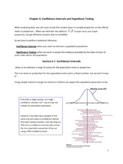
1 Chapter 2: Simple Linear Regression1 The modelThesimple Linear regressionmodel fornobser-vations can be written asyi= 0+ 1xi+ei, i= 1,2, ,n.(1)The designationsimpleindicates that there is onlyone predictor variablex, andlinearmeans thatthe model is Linear in 0and 1. The intercept 0and the slope 1are unknown constants, andthey are both calledregression coefficients;ei sare random errors. For model (1), we have thefollowing (ei) = 0fori= 1,2, ,n, or, equiva-lentlyE(yi) = 0+ var(ei) = 2fori= 1,2, ,n, or, equiva-lently, var(yi)) = (ei,ej) = 0for alli6=j, or, equivalently,cov(yi,yj) = Ordinary Least Square EstimationThemethod of least squaresis to estimate 0and 1so that the sum of the squares of the differ-ence between the observationsyiand the straightline is a minimum, , minimizeS( 0, 1) =n i=1(yi 0 1xi) = XE(Y|X=x) 1=Slope 0=Intercept1 Figure 1.

2 Equation of a straight lineE(Y|X=x) = 0+ least-squares estimators of 0and 1, say 0and 1, must satisfy 2n i=1(yi 0 1xi) = 0(2) 2n i=1(yi 0 1xi)xi= 0(3)Simplifying these two equations yieldsn 0+ 1n i=1xi=n i=1yi 0n i=1xi+ 1n i=1x2i=n i=1yixi(4)Equations (4) are called theleast-squares nor-mal equations. The solution to the normal equa-tions is 1= ni=1xiyi n x y ni=1x2i n x2= ni=1(xi x)(yi y) ni=1(xi x)2=SxySxx, 0= y 1 difference between the observed valueyiand the corresponding fitted value yiis aresidual, , ei=yi yi=yi ( 0+ 1xi), i= 1,2, ,nUsing Forbe s data, we have x= , y= , Sxy= ,Syy= , the parameter estimates are 1=SxySxx= , 0= y 1 x= estimate line, given by either of the equations E(Lpress|temp) = + fit of this line to the data is excellent as shownin Figure (Pressure) 2.

3 Regression for log(pressure) versus Properties of the least-squares estimators and the fit-ted Regression modelIf the three assumptions in section 1 hold, thenthe least squares estimators 0and 1are unbi-ased and have minimum variance among all linearunbiased estimates (best Linear unbiased estima-tors). (The corresponding Gauss-Markov theoremis proved in Appendix).E( 1) = 1,E( 0) = 0,var( 1) = 2 Sxxvar( 0) = 2(1n+ x2 Sxx)There are several other useful properties of theleast squares fit:1. The sum of the residuals in any regressionmodel that contains an intercept 0is alwayszero, that is,n i=1(yi yi) =n i=1 ei= The sum of the observed valuesyiequals thesum of fitted values yi, orn i=1yi=n i=1 The least squares Regression line always passesthrough the centroid (the point ( y, x)) of The sum of the residuals weighted by the cor-responding value of the regressor variable al-ways equals zero, that isn i=1xi ei= The sum of the residuals weighted by the cor-responding fitted value always equals zero, thatis,n i=1 yi ei= 0,or y e= Estimation of 2 The estimate of 2is obtained from the residualsum of squares (SSRes) or sum of squared error(SSE)

4 ,SSRes=n i=1e2i=n i=1(yi yi) related formulas are Regression sum of squares(SSR) and total sum of squares (SST)SSR=n i=1( yi y)2= 1 Sxy,SST=n i=1(yi y) they satisfy the following equation,SST=SSR+ unbiased estimate of 2is 2=SSResn 2= The models in the centered formSuppose we redefine the regressor variablexiasthe deviation from its own average, sayxi Regression model then becomesyi= 0+ 1(xi x) + 1 x+ i= ( 0+ 1 x) + 1(xi x) + i= 0+ 1(xi x) + iIt is easy to show that 0= y, the estimator ofthe slope is unaffected by the transformation, andCov( 0, 1) = Hypothesis testing on the slope and interceptHypothesis testing and confidence intervals (nextsection) require that we make the additional as-sumption that the model errors iare normally dis-tributed.

5 Thus, the complete assumptions are that i N(0, 2).Suppose that we wish to test the hypothesis thatthe slope equals a constant, say 10. The appro-priate hypotheses areH0: 1= 10H1: 16= 10(5)Sinceei N(0, 2), we haveyi N( 0+ 1xi, 2)and 1 N( , 2/Sxx). Therefor,Z0= 1 10 2/Sxx N(0,1)if the null hypothesisH0: 1= 10is true. If 2were known, we could useZ0to test the hypothe-sis (5).If 2is unknown, we know that (1)MSResis anunbiased estimator of 2; (2)(n 2)MSRes/ 2follows a 2n 2distribution; and (3)MSResand 1are independent. Therefore,t0= 1 10 MSRes/Sxx= 1 10se( 1)follows atn 2distribution if the null hypothesisH0: 1= 10is true. The null hypothesis is rejected if|t0|> t /2,n testH0: 0= 00H1: 06= 00,(6)we could use the test statistict0= 0 00 MSRes(1n+ x2 Sxx)= 0 00se( 0).

6 A very important special case of the hypothesisin (5) isH0: 1= 0H1: 16= 0,(7)Failing to reject the null hypothesis implies that thereis no Linear relationship the snowfall data, 1= , andse( 1) = Thus,t= ( 0) = Comparingtwith the critical valuet( ,91) = , we conclude that early and late season snow-falls are The analysis of varianceWe may also use an analysis of variance approachto test significance of Regression . The analysis ofvariance is based on the fundamental analysis ofvariance identity for a Regression model, ,SST=SSR+ 1degrees of freedom be-cause one degree of freedom is lost as a result ofconstraint ni=1(yi y)on the deviationsyi y;SSRhasdfR= 1degree of freedom becauseSSRis completely determined by one parameter,namely, 1;SSReshasdfRes=n 2degrees offreedom because two constraints are imposed onthe deviationsyi yias a result of estimating 0and 1.

7 Note that the degrees of freedom have anadditive property:dfT=dfR+dfResn 1 = 1 + (n 2)We can show: (1) thatSSRes/ 2= (n 2)MSRes/ 2follows a 2n 2distribution; (2) thatif the null hypothesisH0: 1= 0is true, thenSSR/ 2follows a 21distribution; and (3) thatSSResandSSRare independent. By the definition of anFstatistic,F0=SSR/dfRSSRes/dfRes=SSR/1 SSRes/(n 2)=MSRMSR esfollows theF1,n 2distribution. IfF0> F ,1,n 2we reject the null hypothesisH0: 1= 0. Therejection region is single-sided, due to that (Ap-pendix )E(MSRes) = 2, E(MSR) = 2+ 21 Sxx,Source of Sum ofDegrees of MeanF0 Variation SquaresFreedom SquareRegressSSR= 1 Sxy1 MSRMSRMSResResidualSSRes=SST 1 Sxyn 2 MSResTotalSSTn 1 Table 1: Analysis of Variance (ANOVA) for testing significance of regressionthat is, it is likely that the slope 16= 0if the ob-served value ofF0is analysis of variance is summarized in thefollowing analysis of variance for Forbes data is givenSource of Sum of Degrees of MeanF0 Variation Squares Freedom SquareRegress 2.

8 Analysis of Variance (ANOVA) for Forbes Table Coefficient of determinationThe quantityR2=SSRSST= 1 SSResSSTis called the coefficient of determination. For Forbes data,R2= ,and thus the variability in the ob-served values is explained by boiling the below, we list some properties The range ofR2is0 R2 1. If all the j swere zero, except for 0,R2would be zero.(This event has probability zero for continuousdata.) If all they-values fell on the fitted sur-face, that is, ifyi= yi,i= 1,2, ,n, thenR2would be Adding a variablexto the model increases(cannot decrease) the value invariant to a scale change not measure the appropriateness ofthe Linear model, forR2will often be largeeven thoughyandxare nonlinearly Interval estimation in Simple Linear Confidence intervals on 0, 1and 2 The width of these confidence intervals is a mea-sure of the overall quality of the Regression the errors are normally and independently dis-tributed, then the sampling distribution of both 1 1se( 1)and 0 0se( 0)istwithn 2degrees of freedom.

9 Therefore,a100(1 )percent confidence interval on theslope 1is given by 1 t /2,n 2se( 1) 1 1+t /2,n 2se( 1)and a100(1 )percent confidence interval onthe intercept 0is 0 t /2,n 2se( 0) 0 0+t /2,n 2se( 0)Frequency interpretation:If we were to take repeatedsamples of the same size at the samplexlevelsand construct, for example,95%confidence inter-vals on the slope for each sample, then95%ofthose intervals will contain the true value of Forbes data,se( 0) = (1/17 +( )2 )1/2= , andse( 1) = / Sxx= For a90%confidence inter-val,t( ,15) = , and the interval is ( ) 0 + ( ) 0 interval for the slope ( ) 1 + ( ) 1 the errors are normally and independently dis-tributed, then the sampling distribution of(n 1)MSRes/ 2is chi-square with(n 2)degrees of ,P{ 21 /2,n 2 (n 2)MSRes 2 2 /2,n 2}= 1 and consequently a100(1 )percent confidenceinterval on 2is(n 2)MSRes 2 /2,n 2 2 (n 2)

10 MSRes 21 /2,n Interval estimation of the mean responseLetx0be the level of the regressor variable forwhich we wish to estimate the mean response, sayE(y|x0). We assume thatx0is any value of theregressor variable within the range of the originaldata onxused to fit the model. An unbiased pointestimator ofE(y|x0)is E(y|x0) = y|x0= 0+ variance of y|x0isV ar( y|x0) =V ar[ y+ 1(x0 x)] = 2[1n+(x0 x)2 Sxx]since cov( y, 1) = 0. Thus, the sampling distribu-tion of y|x0 E(y|x0) MSRes(1/n+ (x0 x)2/Sxx)istwithn 2degrees of freedom. Consequently,a 100(1 )percent confidence interval on themean response at the pointx=x0is y|x0 t /2,n 2 MSRes(1/n+ (x0 x)2/Sxx) E(y|x0) y|x0+t /2,n 2 MSRes(1/n+ (x0 x)2/Sxx)(8)10 Prediction of new observationsAn important application of the Regression modelis prediction of new observationsycorrespondingto a specified level of the regressor variablex.