Transcription of Chapter 2 Vehicle Dynamics Modeling - Virginia Tech
1 10 Chapter 2 Vehicle Dynamics ModelingThis Chapter provides information on Dynamics Modeling of Vehicle and tire. Thevehicle axis system used throughout the simulation is according to the SAE standard, asdescribed in SAE J670e [18]. According to a brief research study of typical vehiclemodels, a nonlinear three-degree-of-freedom Vehicle model will be used in this derivation of that model including the tire model is discussed first. The equations ofmotion are then converted to a state space form for ease of integration and a Third OrderRunge-Kutta integration routine is used as the integration algorithm. Finally, the vehiclemodel is verified against results from Smith et al. [14] to show its Vehicle Axis SystemThroughout this thesis, the coordinate system used in Vehicle Dynamics Modeling will beaccording to SAE J670e [18] as shown in Figure The x-axis points to the forwarddirection or the longitudinal direction, the y-axis, which represents the lateral direction,is positive when it points to the right of the driver, and the z-axis points to the groundsatisfying the right hand Vehicle Axis System after SAE [18]11In most studies related to handling and directional control, only the X-Y plane ofthe Vehicle is considered.
2 The vertical axis, Z, is often used in the study of ride, pitch,and roll stability type problems. The following list defines relevant definitions for thevariables associated with this direction: forward moving direction of the Vehicle . There are twodifferent ways of looking at the forward direction, one with respect to the Vehicle bodyitself, and another with respect to a fixed reference point. The former is often used whendealing with acceleration and velocity of the Vehicle . The latter is used when thelocation information of the Vehicle with respect to a starting or an ending point direction: sideways moving direction of the Vehicle . Again, there are twoways of looking at the lateral direction, with respect to the Vehicle and with respect to afixed reference point. Researchers often find this direction more interesting than thelongitudinal one since extreme values of lateral acceleration or lateral velocity candecrease Vehicle stability and slip angle: This is equivalent to heading in a given direction but walking atan angle to that direction by displacing each foot laterally as it is put on the ground asshown in Figure The foot is displaced laterally due to the presence of lateral Walking Analogy to Tire Slip Angle after Milliken [19]12 Figure shows the standard tire axis system that is commonly used in tiremodeling.
3 It shows the forces and moments applied to the tire and other importantparameters such as slip angle, heading angle, SAE Tire Axis System after Milliken [19]Body-slip angle: is the angle between the X-axis and the velocity vector thatrepresents the instantaneous Vehicle velocity at that point along the path, as shown inFigure It should be emphasized that this is different from the slip angle associatedwith tires. Even though the concept is the same, each individual tire may have differentslip angle at the same instant in time. Often the body slip angle is calculated as the ratioof lateral velocity to longitudinal Body-Slip Angle after Milliken [19]In order to simplify the Vehicle model so that results of the integration can bequickly calculated, the effects of camber angle, load transfer, and aerodynamics are notincluded in this Vehicle ModelsThere are numerous degrees of freedom associated with Vehicle Dynamics .
4 The mostsimplified Vehicle dynamic model is a two-degree-of-freedom bicycle model,representing the lateral and yaw motions. The idea behind this model is that sometimesit is not necessary or desirable to include the longitudinal direction, because it does notaffect the lateral or yaw stability of the Vehicle . This model, which is easier tounderstand, is often used in teaching purposes. Figure shows the two-degree-of-freedom "baFr Ff r f V yxFigure Two-Degree-of-Freedom ModelA three-degree-of-freedom model adds longitudinal acceleration to the model,therefore enabling one to describe the full Vehicle motion in the X-Y plane. As shown inFigure , the longitudinal velocity, U, and the longitudinal force, Ftf and Ftr, areincluded into the model. This is the model that is used throughout this Three-Degree-of-Freedom Model after Smith [18]In some studies, the rotational degrees of freedom for the front and rear wheelsare added to the model to include the effects of longitudinal slip, as shown in Figure five-degree-of freedom model enables one to perform an in-depth study of tractionand braking forces on handling maneuvers by including the effects of wheel degrees of freedom are also often used in the studies of combined braking andsteering, and braking system controller design, [2,20].
5 15 Figure Rotational Degree of Freedom at Wheel after Smith [18]An eight-degree-of-freedom model no longer assumes symmetry in dynamicbehavior between right and left sides. Rotational degree of freedom for each of the fourtires is considered in this Vehicle model instead of two tires. It also adds a rollingmotion, s, between left and right sides of the Vehicle . This model is often used in thesuspension design or ride comfort analysis, specifically looking at the effects of theseissues with respect to roll and side-to-side load Eight-Degree of Freedom Model after Smith [18] Three-Degree-of-Freedom Vehicle Model DerivationCapturing all the motions of a Vehicle into analytical equations can be quite including more number of elements in the model may increase the model saccuracy, it substantially increases the computation time. This section describes thederivation of the three-degree-of-freedom bicycle model used in this study.
6 It alsoincludes the equations for the front and rear tire slip angles. For this research this is thefirst step in the process, before proceeding to designing an optimization algorithm. Thissection of the Chapter also describes concepts such as tire slip angle, friction ellipse,longitudinal force limits, and state space Equations of MotionThe three degrees of freedom model considered for this study is governed by thefollowing equations:IaP bFbFffr =+ ( )mV VPFFffr( ) +=++( )mVVP P Ffr f( ) +=++( )Referring to Figure , the lateral and longitudinal velocities of the Vehicle withrespect to the fixed coordinate system XYZ can be described as shown in Eqs. ( ) and( )."baFr Ff Ff Fr r f V V yxFigure Three-Degree-of-Freedom Used for Simulation17 sincosxVV= + ( ) cossinyVV=+ ( )WhereF f, F r = lateral tire force on front and rear tires a= Vehicle center of gravity location from front axle b = Vehicle center of gravity location from rear axle m = Vehicle mass I= Vehicle yaw inertiaPf, Pr= longitudinal force on front and rear tiresV ,V = longitudinal/lateral velocity of Vehicle in body reference frame x, y = longitudinal/lateral position of Vehicle in inertial reference frame = steering angle = longitudinal axis in body reference frame = yaw angle = lateral axis in body reference frameThe parameters used for the simulation are shown in Table 1.
7 These parameters arebased on Vehicle specifications provided by The Goodyear Tire and Rubber Company[21].Table Vehicle Parameter Used for Simulation kgInertia (about Z-axis) kgm2 Front Axle to Center of mRear Axle to Center of mHeight Center of Gravity Location Front Tire Slip Angle DerivationFront tire slip angle is a function of front tire steering angle, the longitudinal velocityvector, the lateral velocity vector, and the lateral velocity component due to yaw. illustrates the front tire slip angle, which is mathematically defined as() faVV= + ( )where = steering anglea = center of gravity location from Vehicle rear axle = yaw velocity of vehicleV = lateral velocity of vehicleV = longitudinal velocity of vehicleFigure Front Tire Slip Angle after Milliken [19]Equation ( ), which describes the front tire slip angle formula, assumes that theslip angle is small. It is necessary to determine the front tire slip angle because the Segellateral force tire model is a function of slip angle [7].
8 This tire model will be explained indetails in a later section. The Segel lateral force model will be discussed in Section Rear Tire Slip Angle DerivationThe rear tire slip angle is a result of a combination of the ratio of the longitudinalvelocity vector and the lateral velocity vector, and the lateral velocity component due toyaw. Figure illustrates the rear tire slip angle.() rbVV= ( )whereb = center of gravity location from Vehicle rear axle = yaw velocity of vehicleV = lateral velocity of vehicleV = longitudinal velocity of vehicleFigure Rear Tire Slip Angle after Milliken [19]Equation ( ), which describes the rear tire slip angle formula, assumes that theslip angle is small. It is necessary to determine the rear tire slip angle because the Segellateral force tire model is a function of slip angle [7]. This tire model will be explained indetails in a later section. The Segel lateral force model will be described in Section Longitudinal (Traction/Braking) ForceThe traction force limit for a front wheel drive Vehicle is calculated as the following,[22].
9 FWblhlxtmax,=+ 1 ( )The maximum braking force for an independent suspension, front wheel drivevehicle is calculated as the following, [22].()FWlahxbmax,=+ ( )whereFxtmax, = maximum tractive forceF = maximum braking force = friction coefficienta = center of gravity location from front axleb = center of gravity location from rear axleW = Vehicle weightl = Vehicle wheelbaseh = center of gravity location from The values of Eq. ( ) and ( ) are calculated to be N and Nrespectively, using the parameters in Table 1. Throughout this study, however, thetraction force limit and the braking force limit are set to 5000 N and -5000 N,respectively. This enables the use of one variable to describe the constraint of thelongitudinal force in the optimal control algorithm. This is explained in more details inChapter Segel Lateral Force ModelThere are several lateral force models that have been derived in the past.
10 They rangefrom using a collective set of tire performance data, to determining an empirical lateralforce model, to analytical tire models derived from differential equations describing thedeformation of tire structure [7]. The lateral force model selected for this research is theSegel Model. This model was developed in the early 1970's. There are newer modelsthat can be used to describe the lateral force of a tire. However, Segel model is fairlyeasy to use and has relatively small computation time [7]. It is a function of the slipangle, cornering stiffness, tire vertical load, friction coefficient, and longitudinal force, asdescribed = + + ~~~~3271322222i = f, r( )~ iiizicF=i = f, r( )() faVV= + ( )() rbVV= ( )()FmgbPP habzffr= ++( )()FmgaPP habzrfr=+++( )where22c = cornering stiffness of front and rear tiresF= normal tire load on front and rear tiresF= lateral tire force on front and rear tiresg = gravitational accelerationh = height of the center of gravitya = front axle to center of gravity distanceb = rear axle to center of gravity distancem = Vehicle mass = friction coefficient= slip angle of front and rear tiresP= longitudinal force of front and rear tiresV = longitudinal & lateral velocity in body reference framex, y = longitudinal & lateral position in inertial reference frame =fzffff,,,,,,cFFPV rzrrrr steering angle = yaw angle = yaw velocity Friction Ellipse ConceptThis topic is discussed in this section because it is related to the two previous topics,longitudinal force and lateral force.