Transcription of CHAPTER 5 - CURVE FITTING
1 CHAPTER 5 CURVE FITTINGCURVE FITTINGP resenter: Dr. Zalilah Sharer 2018 School of Chemical and Energy EngineeringUniversiti Teknologi Malaysia23 September 2018 TOPICSL inear regression (exponential model, power equation and saturation growth rate equation)Polynomial Regression Polynomial Interpolation (Linear interpolation, Quadratic Interpolation, Newton DD)Lagrange InterpolationCurve FITTING CURVE fittingdescribes techniques to fit curves at points between the discrete values to obtain intermediate estimates. Two general approaches for CURVE FITTING :a)Least Squares Regression -to fits the shape or a)Least Squares Regression -to fits the shape or general trend by sketch a best line of the data without necessarily matching the individual points (figure , pg 426).- 2 types of FITTING :i) Linear Regressionii) Polynomial RegressionFigure shows sketches developed from same set of data by 3 ) least-squares regression -did not attempt to connect the point, but characterized the general upward trend of the data with a straight lineb) Linear interpolation -Used straight-line segments or linear interpolation to connect the points.
2 Very common practice in engineering. If the values are close to being linear, such approximation provides estimates that are adequate for many engineering adequate for many engineering calculations. However, if the data is widely spaced,significant errorscan be introduced by such linear ) Curvilinear interpolation -Used curves to try to capture suggested by the data. Our goal here to develop systematic and objective method deriving such ) Least-square Regression : i) Linear Regression Is used to minimize the discrepancy/differences between the data points and the CURVE plotted. Sometimes, polynomial interpolation is inappropriate and may yield unsatisfactory results when used to predict intermediate values (see Fig. , pg 455). , pg 455).Fig. a): shows 7 experimentally derived data points exhibiting significant variability. Data exhibiting significant FittingLinear Regression is FITTING a best straight line through the mathematical expression for the straight line is:y = a0+a1x+eEq , a1-slopea-intercepta0 -intercepte -error, or residual, between the model and the observationsRearranging the eq.
3 Above as:e = y - a0 - a1xThus, the error or residual, is the discrepancy between the true value yand the approximate value, a0+a1x, predicted by the linear for a best Fit To know how a best fit line through the data is by minimize the sum of residual error, given by ;where; n : total number of points == =niiiniixaaye1101)(----- Eq A strategy to overcome the shortcomings: The sum of the squares of the errorsbetween the measured yand the ycalculated with the linear model is shown in Eq ; === = ==niniiielimeasurediniirxaayyyeS112102mo d,,12)()(----- Eq fit for a straight line To determine values for aoand a1, i) differentiate equation with respect to each coefficient, ii) setting the derivations equal to zero (minimize Sr), iii) set ao= give equations and , called as normal equations, (refer text book)which can be solved simultaneously for a1and ao;()xayaxxnyxyxnaiiiiii10221 = = ----- Eq Eq 1 Use least-squares regression to fit a straight line Two criteria for least-square regression will provide the best estimates of aoand a1called maximum likelihood principlein statistics:i.
4 The spread of the points around the line of similar magnitude along the entire range of the The distribution of these points about the line is normal. If these criteria are met, a standard deviation for the regression line is given by equation:---------- Eq. : standard error of estimate y/x : predicted value of ycorresponding to a particular value of xn -2 : two data derived estimates aoand a1were used to compute Sr(we have lost 2 degree of freedom) 2 =nSSrxy Equation is derived from Standard Deviation (Sy) about the mean :-------- ( , pg 442 )-------- ( , pg 442 )1 =nSSty =2)(yySitSt: total sum of squares of the residuals between data points and themean. Just as the case with the standard deviation, the standard error of the estimate quantifies the spread of the data. Estimation of error in summary1. Standard error of the estimate = =2)(1yySnSSitty----- ( , pg 442 )----- ( , pg 442 ) error of the estimatewhere, y/x designates that the error is for a predict value of y corresponding to a particular value of )(112102 = == ==nrSSxaayeiSxyniniir----- Eq Eq Determination coefficienttrtSSSr =2----- Eq Correlation coefficient = =2222)()())((@iiiiiiiitrtyynxxnyxyxnrSSS r----- Eq 2 Use least-squares regression to fit a straight line the standard deviation (Sy), the standard error of estimate (Sy/x) and the correlation coefficient (r) for data above (use Example 1 result) Work with your buddy and lets do Quiz 1 Use least-squares regression to fit a straight line to.
5 Compute the standard error of estimate (Sy/x) and the correlation coefficient (r) 2 Compute the standard error of the estimate and the correlation of Nonlinear Relationships Linear regression provides a powerful technique for FITTING the best line to data, where the relationship between the dependent and the relationship between the dependent and independent variables is linear. But, this is not always the case, thus first step in any regression analysis should be to plot and visually inspect whether the data is a linear model or : a) data is ill-suited for linear regression,b) parabola is preferable. Linear regression is predicated on the fact that therelationship between the dependent andindependent variables is linear - this is not alwaysthe Relationships Three common examples are:exponential :y= 1e 1xpower :y= 2x 2saturation - growth - rate :y= 3x 3+x One option for finding the coefficients for a nonlinear fit is to linearize it.
6 For the three common models, this may involve taking logarithms or inversion:Linearization of Nonlinear Relationships ModelNonlinearLinearizedexponential :y= 1e 1xln y=ln 1+ 1xpower :y= 2x 2log y=log 2+ 2logxsaturation - growth - rate :y= 3x 3+x1y=1 3+ 3 31x After linearization, Linear regression can be applied to determine the linear relation. For example, the linearized exponential equation: Linearization of Nonlinear Relationships xyln ln +=xy11ln ln +=yxa10aFigure : Type of polynomial equations and their linearizedversions, respectively. Fig. , pg 453 shows population growth of radioactive decay (a) : theexponential model------ ( )xey11 = 1, 1: constants, 1 0 This model is used in many fields of engineering to characterize increase : 1positiveQuantities decrease : 1negative Fit an exponential model y= a 2 Solution Linearized the model into;ln y = ln a + bxy = a0 + a1x ----- (Eq. ) Build the table for the parameters used in eqs and , as in example , pg yixi2(xi)(ln yi) ))(ln( ==== ) () )(6() )( () )(6( )()(ln))(ln(2221= = == ) )( ( = == += +=bxeay= = Straight-line:Exponential:Figure : Type of polynomial equations and their linearizedversions, Equation Equation ( ) can be linearized by taking base-10 logarithm to yield.
7 -------- ( )--------( )xyxylogloglog22 +==--------( ) A plot of log yversus log xwill yield a straight line with slope of 2and an intercept of log +=Example 4 Linearization of a Power equation and fit equation ( ) to the data in table below using a logarithmic transformation of the (logxi)2(logxi)(logyi) ))(log( )( ====yxyxxyxnniniiiiniiniib=n (logxi)(logyi) ( logxi)( logyi)n (logxi)2 ( logxi)2b=(5)( ) ( )( )(5)( ) ( )2= + = += ) )( ( )(logloglog = = =axbyaStraight-line:bxay= = Power: Fig. a), pg 455, is a plot of the original data in its untransformed state, while fig. b) is a plot of the transformed data. The intercept, log = The intercept, log 2= , and by taking the antilogarithm, 2= The slope is 2= , consequently, the power equation is : y = : Type of polynomial equations and their linearizedversions, growth rate equation Equation ( ) can be linearized by inverting it to yield:------- ( )-------( )333111 +=xy +=xxy33 -------( ) A plot of 1/yversus 1/xwill yield a straight line with slope of 3/ 3and an intercept of1/ 3 In their transformed forms, these models are fit using linear regression in order to evaluate the constant coefficients.
8 This model well-suited for characterizing population growth under limiting xyExample 5 Linearization of a saturation-growth rate equation to the data in table 2 468 = === ==== == ==yxiiiiixiyi1/ xi1/ yi(1/xi)2(1/ xi)(1/yi) ) () )(7() )( () )(7()1(11111222= = = ) )( ( = = axabyaxabay111+= += Straight-line:xy += )2)( ( == =babaa += :Lets do Quiz 3 Fit a power equation and saturation growth rate equation : a) data is ill-suited for linear regression, b) parabola is Regression Another alternative is to fit polynomials to the data using polynomial regression. The least-squares procedure can be readily extended to fit the data to a higher-order polynomial. For example, to fit a second order polynomial or quadratic: The sum of the squares of the residual is:where n= total number of points = =niiiirxaxaayS122210)(exaxaay+++=2210 Then, taking the derivative of equation ( ) with respect to each of the unknown coefficients, ao, a1,and, a2of the polynomial, as in: = =)(2)(22210122100iiiiriiirSxaxaayxaSxaxa ayaS Setting the equations equal to zero and rearrange to develop set of normal equations and by setting ao= =++=++=++iiiiiiiiiiiiiyxaxaxaxyxaxaxaxya xaxan2241302231202210)()()()()()()()()( =)(2221022iiiirxaxaayxaS ----- The above 3 equations are linear with 3 unknowns coefficients (ao, a1,and, a2) which can be calculated directly from observed data.
9 In matrix form: The two-dimensional case can be easily extended to an mth-order = iiiiiiiiiiiiiyxyxyaaaxxxxxxxxn2210432322 The two-dimensional case can be easily extended to an m-order polynomial as: Thus, standard error for mth-order polynomial :exaxaxaaymm+++++=..2210)1(/+ =mnSSrxy----- 6 Fit a second order polynomial to the data in the first 2 columns of table :xiyixi2xi3xi4xi From the given data:m = 2 xi= 15 xi4= 979y= = 6 yi= xiyi= xi3= 225x= xi2= 55 xi2yi= Therefore, the simultaneous linear equations are: Solving these equations through a technique such as Gauss = iiiiiiiiiiiiiyxyxyaaaxxxxxxxxn2310432322 = Solving these equations through a technique such as Gauss elimination gives:ao= , a1= , and a2= Therefore, the least-squares quadratic equation for this case is:y = + + To calculate stand sr, build table for columns 3 and (yi- y )2(yi-ao-a1xi-a2xi2) )( )(22210= == =iiiritxaxaaySyySThe standard error (regression polynomial) )12( )1(=+ =+ =mnSSrxy The correlation coefficient can be calculated by using equations and , respectively.
10 Therefore,r2= (S S) / S= ( ) / = =2222)()())((@iiiiiiiitrtyynxxnyxyxnrSSS rtrtSSSr =2 Therefore,r2= (St Sr) / St= ( ) / The correlation coefficient is, r = The results indicate that of the original uncertainty has been explained by the model. This result supports the conclusion that the quadratic equation represents an excellent fit, as evident from : fit of a second-order polynomialTOPICSP olynomial Interpolation (Linear interpolation, Quadratic Interpolation, Newton DD)Lagrange InterpolationSpline InterpolationInterpolation Polynomial Interpolation is a common method to determine intermediate values between data points. General equation for nthorder polynomial is: Polynomial interpolation consists of determining the unique nth-order polynomial that fits n+1data point. For n+1data points, there is only one polynomial of order nthat nnxaxaxaaxf+++=..)(2210----- For n+1data points, there is only one polynomial of order nthat passes through all the points.