Transcription of Chapter 6: Continuous Probability Distributions
1 Chapter 6: Continuous Probability Distributions 175 Chapter 6: Continuous Probability Distributions Chapter 5 dealt with Probability Distributions arising from discrete random variables. Mostly that Chapter focused on the binomial experiment. There are many other experiments from discrete random variables that exist but are not covered in this book. Chapter 6 deals with Probability Distributions that arise from Continuous random variables. The focus of this Chapter is a distribution known as the normal distribution , though realize that there are many other Distributions that exist. A few others are examined in future chapters. Section : Uniform distribution If you have a situation where the Probability is always the same, then this is known as a uniform distribution . An example would be waiting for a commuter train.
2 The commuter trains on the Blue and Green Lines for the Regional Transit Authority (RTA) in Cleveland, OH, have a waiting time during peak hours of ten minutes ("2012 annual report," 2012). If you are waiting for a train, you have anywhere from zero minutes to ten minutes to wait. Your Probability of having to wait any number of minutes in that interval is the same. This is a uniform distribution . The graph of this distribution is in figure # Figure # : Uniform distribution Graph Suppose you want to know the Probability that you will have to wait between five and ten minutes for the next train. You can look at the Probability graphically such as in figure # Chapter 6: Continuous Probability Distributions 176 Figure # : Uniform distribution with P(5 < x < 10) How would you find this Probability ?
3 Calculus says that the Probability is the area under the curve. Notice that the shape of the shaded area is a rectangle, and the area of a rectangle is length times width. The length is 10!5=5 and the width is The Probability is P5<x<10()= *5= , where and x is the waiting time during peak hours. Example # : Finding Probabilities in a Uniform distribution The commuter trains on the Blue and Green Lines for the Regional Transit Authority (RTA) in Cleveland, OH, have a waiting time during peak rush hour periods of ten minutes ("2012 annual report," 2012). a.) State the random variable. Solution: x = waiting time during peak hours b.) Find the Probability that you have to wait between four and six minutes for a train. Solution: P4<x<6()=6!4()* c.) Find the Probability that you have to wait between three and seven minutes for a train.
4 Solution: P3<x<7()=7!3()* d.) Find the Probability that you have to wait between zero and ten minutes for a train. Solution: P0<x<10()=10!0()* Chapter 6: Continuous Probability Distributions 177 e.) Find the Probability of waiting exactly five minutes. Solution: Since this would be just one line, and the width of the line is 0, then the Px=5()=0* Notice that in example # , the Probability is equal to one. This is because the Probability that was computed is the area under the entire curve. Just like in discrete Probability Distributions , where the total Probability was one, the Probability of the entire curve is one. This is the reason that the height of the curve is In general, the height of a uniform distribution that ranges between a and b, is 1b!a. Section : Homework 1.) The commuter trains on the Blue and Green Lines for the Regional Transit Authority (RTA) in Cleveland, OH, have a waiting time during peak rush hour periods of ten minutes ("2012 annual report," 2012).
5 A.) State the random variable. b.) Find the Probability of waiting between two and five minutes. c.) Find the Probability of waiting between seven and ten minutes. d.) Find the Probability of waiting eight minutes exactly. 2.) The commuter trains on the Red Line for the Regional Transit Authority (RTA) in Cleveland, OH, have a waiting time during peak rush hour periods of eight minutes ("2012 annual report," 2012). a.) State the random variable. b.) Find the height of this uniform distribution . c.) Find the Probability of waiting between four and five minutes. d.) Find the Probability of waiting between three and eight minutes. e.) Find the Probability of waiting five minutes exactly. Chapter 6: Continuous Probability Distributions 178 Section : Graphs of the Normal distribution Many real life problems produce a histogram that is a symmetric, unimodal, and bell-shaped Continuous Probability distribution .
6 For example: height, blood pressure, and cholesterol level. However, not every bell shaped curve is a normal curve. In a normal curve, there is a specific relationship between its height and its width. Normal curves can be tall and skinny or they can be short and fat. They are all symmetric, unimodal, and centered at , the population mean. Figure # shows two different normal curves drawn on the same scale. Both have =100 but the one on the left has a standard deviation of 10 and the one on the right has a standard deviation of 5. Notice that the larger standard deviation makes the graph wider (more spread out) and shorter. Figure # : Different Normal distribution Graphs Every normal curve has common features. These are detailed in figure # Figure # : Typical Graph of a Normal Curve The center, or the highest point, is at the population mean.
7 The transition points (inflection points) are the places where the curve changes from a hill to a valley . The distance from the mean to the transition point is one standard deviation, !. The area under the whole curve is exactly 1. Therefore, the area under the half below or above the mean is Chapter 6: Continuous Probability Distributions 179 The equation that creates this curve is fx()=1!2"e#12x# !$%&'()2. Just as in a discrete Probability distribution , the object is to find the Probability of an event occurring. However, unlike in a discrete Probability distribution where the event can be a single value, in a Continuous Probability distribution the event must be a range. You are interested in finding the Probability of x occurring in the range between a and b, or Pa!x!b()=Pa<x<b(). Calculus tells us that to find this you find the area under the curve above the interval from a to b.
8 Pa!x!b()=Pa<x<b() is the area under the curve above the interval from a to b. Figure # : Probability of an Event Before looking at the process for finding the probabilities under the normal curve, it is somewhat useful to look at the Empirical Rule that gives approximate values for these areas. The Empirical Rule is just an approximation and it will only be used in this section to give you an idea of what the size of the probabilities is for different shadings. A more precise method for finding probabilities for the normal curve will be demonstrated in the next section. Please do not use the empirical rule except for real rough estimates. The Empirical Rule for any normal distribution : Approximately 68% of the data is within one standard deviation of the mean. Approximately 95% of the data is within two standard deviations of the mean.
9 Approximately of the data is within three standard deviations of the mean. Chapter 6: Continuous Probability Distributions 180 Figure # : Empirical Rule Be careful, there is still some area left over in each end. Remember, the maximum a Probability can be is 100%, so if you calculate 100%! you will see that for both ends together there is of the curve. Because of symmetry, you can divide this equally between both ends and find that there is in each tail beyond the 3!. Chapter 6: Continuous Probability Distributions 181 Section : Finding Probabilities for the Normal distribution The Empirical Rule is just an approximation and only works for certain values. What if you want to find the Probability for x values that are not integer multiples of the standard deviation? The Probability is the area under the curve.
10 To find areas under the curve, you need calculus. Before technology, you needed to convert every x value to a standardized number, called the z-score or z-value or simply just z. The z-score is a measure of how many standard deviations an x value is from the mean. To convert from a normally distributed x value to a z-score, you use the following formula. z-score z=x! " where = mean of the population of the x value and ! = standard deviation for the population of the x value The z-score is normally distributed, with a mean of 0 and a standard deviation of 1. It is known as the standard normal curve. Once you have the z-score, you can look up the z-score in the standard normal distribution table. The standard normal distribution , z, has a mean of =0 and a standard deviation of !=1. Figure # : Standard Normal Curve Luckily, these days technology can find probabilities for you without converting to the z-score and looking the probabilities up in a table.