Con dence intervals and hypothesis tests - mit.edu

1 Chapter 2 Confidence intervals and hypothesis testsThis chapter focuses on how to draw conclusions about populations from sample data. We llstart by looking at binary data ( , polling), and learn how to estimate the true ratio of 1sand 0s with confidence intervals , and then test whether that ratio is significantly differentfrom some baseline value using hypothesis testing. Then, we ll extend what we ve learnedto continuous measurements. Binomial dataSuppose we re conducting a yes/no survey of a few randomly sampled people1, and we wantto use the results of our survey to determine the answers for the overall population. The estimatorThe obvious first choice is just the fraction of people who said yes. Formally, suppose wehavensamplesx1.

2 ,xnthat can each be 0 or 1, and the probability that eachxiis 1isp(in frequentist style, we ll assumepis fixed but unknown: this is what we re interestedin finding). We ll assume our samples areindendepent and identically distributed ( ),meaning that each one has no dependence on any of the others, and they all have the sameprobabilitypof being 1. Then our estimate forp, which we ll call p, or p-hat would be p=1nn i= that pis arandomquantity, since it depends on the random quantitiesxi. In statisticallingo, pis known as anestimatorforp. Also notice that except for the factor of 1/ninfront, pis almost a binomial random variable (that is, (n p) B(n,p)). We can compute itsexpectation and variance using the properties we reviewed:E[ p] =1nnp=p,( )var[ p] =1n2np(1 p) =p(1 p)n.

3 ( )1We ll talk about how to choose and sample those people in Chapter for Research ProjectsChapter 2 Since the expectation of pis equal to the true value of what pis trying to estimate (namelyp),we say that pis anunbiasedestimator forp. Reassuringly, we can see that another goodproperty of pis that its variance decreases as the number of samples increases. Central Limit TheoremTheCentral Limit Theorem, one of the most fundamental results in probability theory,roughly tells us that if we add up a bunch of independent random variables that all have thesame distribution, the result will be approximately can apply this to our case of a binomial random variable, which is really just the sum ofa bunch of independent Bernoulli random variables.

4 As a rough rule of thumb, ifpis closeto , the binomial distribution will look almost Gaussian withn= 10. Ifpis closer or we ll need a value closer ton= 50, and ifpis much closer to 1 or 0 than that, aGaussian approximation might not work very well until we have much more is useful for a number of reasons. One is that Gaussian variables are completely specifiedby their mean and variance: that is, if we know those two things, we can figure out everythingelse about the distribution (probabilities, etc.). So, if we know a particular random variableis Gaussian (or approximately Gaussian), all we have to do is compute its mean and varianceto know everything about it. Sampling DistributionsGoing back to binomial variables, let s think about the distribution of p(remember that thisis a random quantity since it depends on our observations, which are random).

5 Figure thesampling distributionof pfor a case where we flip a coin that we hypothesizeis fair ( the true valuepis ). There are typically two ways we use such samplingdistributions: to obtainconfidence intervalsand to performsignificance tests . Confidence intervalsSuppose we observe a value pfrom our data, and want to express how certain we are that pis close to the true parameterp. We can think about how often therandomquantity pwillend up within some distance of thefixed but unknownp. In particular, we can ask for aninterval around pfor any sample so thatin95%of samples, the true meanpwill lie insidethis interval. Such an interval is called aconfidence interval. Notice that we chose thenumber 95% arbitrarily: while this is a commonly used value, the methods we ll discuss canbe used for any confidence ve established that the random quantity pis approximately Gaussian with meanpandvariancep(1 p)/n.

6 We also know from last time that the probability of a Gaussian randomvariable being within about 2 standard deviations of its mean is about 95%. This meansthat there s a 95% chance of pbeing less than 2 p(1 p)/naway fromp. So, we ll define2 Statistics for Research ProjectsChapter (a) The sampling distribution of the estimator the distribution of values for pgiven a fixedtrue valuep= (b) The 95% confidence interval for a particularobserved pof (with a true value ofp= ).Note that in this case, the interval contains thetrue valuep. Whenever we draw a set of samples,there s a 95% chance that the interval that we getis good enough to contain the true interval p 2 coeff. p(1 p)n std. ( )With probability 95%, we ll get a pthat gives us an interval if we wanted a 99% confidence interval?

7 Since pis approximately Gaussian, its prob-ability of being within 3 standard deviations from its mean is about 99%. So, the 99%confidence interval for this problem would be p 3 coeff. p(1 p)n std. ( )We can define similar confidence intervals , where the standard deviation remains the same,but the coefficient depends on the desired confidence. While our variables being Gaussianmakes this relationship easy for 95% and 99%, in general we ll have to look up or have oursoftware compute these , there s a problem with these formulas: they requires us to knowpin order to computeconfidence intervals ! Since we don t actually knowp(if we did, we wouldn t need a confidenceinterval), we ll approximate it with p, so that ( ) becomes p 2 p(1 p)n.

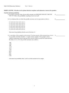
8 ( )This approximation is reasonable if pis close top, which we expect to normally be the the approximation is not as good, there are several more robust (but more complex) waysto compute the confidence for Research ProjectsChapter : Multiple 95% confidence intervals computed from different sets of data, each with thesame true parameterp= (shown by the horizontal line). Each confidence interval representswhat we might have gotten if we had collected new data and then computed a confidence intervalfrom that new data. Across different datasets, about 95% of them contain the true interval. But,once we have a confidence interval, we can t draw any conclusions about where in the interval thetrue value s important not to misinterpret what a confidence interval is!

9 This interval tells us nothingabout thedistributionof the true parameterp. In fact,pis a fixed ( , deterministic)unknown number! Imagine that we samplednvalues forxiand computed palong with a95% confidence interval. Now imagine that we repeated this whole process a huge numberof times (including sampling new values forxi). Then about 5% of the confidence intervalsconstructed won t actually contain the truep. Furthermore, ifpis in a confidence interval,we don t know where exactly within the , adding an extra 4% to get from a 95% confidence interval to a 99% confidenceinterval doesn t mean that there s a 4% chance that it s in the extra little area that youadded! The next example illustrates summary, a 95% confidence interval gives us a region where, had we redone the surveyfrom scratch, then 95% of the time, the true valuepwill be contained in the interval.

10 Thisis illustrated in Figure hypothesis testingSuppose we have a hypothesized or baseline valuepand obtain from our data a value pthat ssmaller thanp. If we re interested in reasoning about whether pis significantly smallerthanp, one way to quantify this would be to assume the true value werepand then computethe probability of getting a value smaller than or as small as the one we observed (we cando the same thing for the case where pis larger). If this probability is very low , we mightthink the hypothesized valuepis incorrect. This is thehypothesis testing begin with anull hypothesis , which we callH0(in this example, this is the hypothesisthat the true proportion is in factp) and analternative hypothesis , which we callH1orHa(in this example, the hypothesis that the true mean is significantly smaller thanp).