Chapter 7 Non-linear Seismic Response of Structures

1 238 Chapter 7 Non-linear Seismic Response of Structures Introduction As per the conventional earthquake-resistant design philosophy, the Structures are designed for forces, which are much less than the expected design earthquake forces. Hence, when a structure is struck with severe earthquake ground motion, it undergoes inelast ic de format ions. Even though the structure may not collapse but the damages can be beyond repairs. In reinforced cement concrete (RCC) Structures , a structural system can be made ductile, by providing reinforcing steel according to the IS:13920-1993 code. A sufficiently ductile structural system undergoes large deformations in the inelastic regio n. In order to understand the complete behaviour of Structures , time history analysis of different Single Degree of Freedom (SDOF) and Multi Degree of Freedom (MDOF) Structures having Non-linear characteristics is required to be performed.

2 The results of time history analysis, Non-linear analysis of these Structures will help in understanding their true behavior. From the results, it can be predicted, whether the structure will not collapse / partially collapse or totally collapse. In this Chapter , the modeling of SDOF and MDOF Structures having Non-linear characteristics for Seismic Response analysis is carried out. The push over analysis of the RCC building is also presented. Non-linear Force-Deformation Behavior The structural systems which have linear inertia, damping and restoring forces, are analysed by linear methods. Whenever, the structural system has any or all of the three reactive forces ( inertia, damping and stiffness) having Non-linear variation with the Response parameters, namely displacement, velocity, and acceleration; a set of Non-linear differential equations is evolved. To obtain the Response , these equations need be solved.

3 The most common non-linearity is the stiffness and the damping non-line arit y. The stiffness non-linearity co mpr ises of two type s namely the geometric non-linearity and the material non-linearity. For the material non-linearity, restoring action shows a hysteretic behavior under cyclic loading. For the geometric non-linearity, no such hysteretic behavior is exhibited. During unloading, the load deformation path follows that of the loading. Figure (a) shows 239 the case of load deformation behavior of the non-hysteretic type. Figure (b) shows the hysteretic behavior of a Non-linear restoring force under cyclic loading (material non-linearity). Damping non-linearity may be encountered in dynamic problems associated with structural control, offshore Structures , and aerodynamics of Structures . Most of the damping non-linearities are of a non-hysteretic type.

4 Most Structures under earthquake excitation undergo yielding. Hence, it is necessary to discuss material non-linearity exhibiting hysteretic behavior. For structural systems having linear behaviour (when subjected to weak ground mot ions) of inertial forces, spring elastic forces and linear damping characteristics, linear methods of analysis can be employed. Displacement, velocity and acceleration are important Response parameters of any structural system. When any or all of the reactive forces, viz. inertia force / spring force or damping force has nonlinear variation with the Response parameters, the analysis involves Non-linear differential equations. Solution of these equations will give the Response of the system. The popular method to obtain the Response is Newmark s Beta method. Figure (a) Non-linear restoring force for geometrical non-linearity (non-hysteretic type) and (b) Non-linear restoring forces (hysteretic type) Displacement Force Displacement Force 240 7.

5 3 Non-linear Analysis of SDOF system Consider a SDOF system having Non-linear damping and stiffness characteristics as shown in the Figure Figure Non-linear SDOF system and its free body diagram. For the SDOF system, the equation of motion in the incremental form is expressed as ii ti tiggmx c x k xmx + + = ( ) where m is the mass of the SDOF system, tc is the initial tangent damping coefficient and tkis the initial tangent stiffness at the beginning of the time step, respectively. The so lution of the equation of motion for the SDOF system is obtained using the numerical integration technique. The incremental quantities in the equation ( ) are the change in the responses from time ti to ti+1 given by 1111 1 iiiiiiiiii iiii igg gxxxxxxxxxt ttxx x+++++ = = = = = ( ) Assuming the linear variation of acceleration over a small time interval, it the incremental acceleration and velocity (refer Section Newmark s Beta Method) are expressed as 266 3iiiiiixxxxtt = ( ) gx m kt ct x ()gmx x+ sF dF m 241 3 3 2iiiiiitxxxxt = ( ) Substituting ix and ix in equation ( ) and solving for theix will give effieffpxk = ( ) where effp and effkare the incremental force and incremental stiffness during the ith time step respectively expressed as.

6 6 2 22iieffgtitiitpmxm cxmcxt = +++ + ( ) 263 effttiikmcktt= ++ ( ) Knowing theix , determine ix fro m equa t ion ( ). At time, t = ti+1, the displacement and velocity can be determined as 11 i iii iix xxx xx++= + = + ( ) The acceleration at time, t = ti+1 is calculated by considering equilibrium of the system (refer Figure ) to avoid the accumulation of the unbalanced forces 1 1111 F i iiig dsxmxFm++++ = ( ) where 1 Fid+ and 1isF+ denote the damping and stiffness/restoring force at time, ti+1, respectively. While obtaining the above so lut ion, it is assumed that the damping and restoring force non-linearities follow the specified path during loading and unloading condition. Elasto-plastic Material Behavior For the elasto-plast ic material behavior, tc is assumed to be constant. The stiffness matrix tkis taken either as k or zero depending upon whether the system is elastically loaded and unloaded or plastically deformed.

7 When the system enters from elast ic to plast ic state or vice-versa, the stiffness varies within the time step. Due to variation of stiffness with respect to time, the system no more remains in equilibrium. 242 If the system is elastic at the beginning of the time step and remains elastic at the end of the time step, then the computation is not changed 1isFQ+< ( ) and the computations for the next time step start. In equation ( ),Qis the yield force. The system enters into plastic state from elastic state as soon as 1isFQ+= ( ) Normally, it is not possible to have the scenario that at time, ti+1, the spring force is just equal to the yield force. However, this can be archived by reduc ing the time interval of the computation.

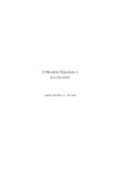
8 Once the system enters into the plastic state, it continues to remain in that state until the incremental displacement and the stiffness force are in the same direction. Thus, the plastic state exists until 10isiFx+ > ( ) When the velocity at the end of the time interval changes the sign then the unloading takes place. Thus, the system changes from plastic to elastic state when 10isiFx+ < ( ) The system remains in the elastic state until equation ( ) is satisfied otherwise, it will change from elastic to plastic state. 243 Example 7. 1 Consider an elasto-plastic SDOF system having mass = 1 kg, elastic stiffness = N/m and damping constant = Determine the displacement Response of the system under the El-Centro, 1940 motion for (i) yield displacement = and (ii) yield displacement = Solution: Based on the method developed in the Section , a computer program is written in the FORTAN language and the Response of the SDOF system with the above parameters and elasto-plast ic behavior under El-Centro, 1940 earthquake motion is obtained.

9 The time period of the system based on the elastic stiffness is 1 sec and the damping ratio is The time variation of displacement and spring force of the system is plotted in Figures and for the yield displacement, q = and , respectively. The salient values of the maximum Response of the system are summarized as below: Response quantity q = q = Maximum displacement (m) Maximum Stiffness force (N) Time of change of first elastic to plastic state sec sec Time of change of first plastic to elastic state sec 2. 02 sec Maximum elastic deflection (refer Example ) m 244 Figure 7. 3 Response of elasto-plast ic SDOF system with yield displacement of 245 Figure 7. 4 Response of elasto-plast ic SDOF system with yield displacement of 246 7. 4 Non-linear Force-Deformation Behaviour using Wen s Equation Wen (1976) proposed the equation for modeling Non-linear hysteretic force-de format ion behavior, in which the force, Fs is given by 0(1)sFk xQZ= + ( ) where k0 is the initial stiffness; is an inde x, which represents the ratio of post to pre-yielding stiffness; x is the relative displacement; Q is the yield strength; and Z is a non-dimensional hysteretic component satisfying the following Non-linear first order differential equation expressed as 1(, )nndZqx Z Zx ZAxg x Zdt = + = ( ) where , , A and n are the dimensionless parameters which control the shape of the hysteresis loop; q is the yield displacement; and x is the relative velocity.

10 The parameter n is an integer constant, which controls the smoothness of transition from elast ic to plast ic state. Various parameters of the Wen s equation are selected in such a way that predicted Response from the model closely matches with the experimental results. In order to solve, the equation of motion of a system in the incremental form using the Newmark s step-by-step method will require the incremental force (refer equation ( )) which is given by 0(1)sFk xQZ = + ( ) The above equation involves the incremental displacement component, Z which can be obtained by solving the differential equation ( ) using the fourth order Runge-Kutta method by 0 1 23226K K KKZ+++ = ( ) 0( , )/tKtg x Zq= ( ) /210(,/ 2) /tttKtg xZKq+ = + ( ) /221(,/ 2) /tttKtg xZKq+ = + ( ) 247 32(,)/tt tKtg xZKq+ = + ( ) It is to be noted that the above solut ion requires the velocity of the system at time, t+ t/2 and t+ t which are not known initially.