Transcription of Chapter 8 Natural and Step Responses of RLC Circuits
1 Chapter 8. Natural and Step Responses of RLC Circuits The Natural Response of a Parallel RLC. circuit The Step Response of a Parallel RLC. circuit The Natural and Step Response of a Series RLC circuit 1. Key points What do the response curves of over-, under-, and critically-damped Circuits look like? How to choose R, L, C values to achieve fast switching or to prevent overshooting damage? What are the initial conditions in an RLC circuit ? How to use them to determine the expansion coefficients of the complete solution? Comparisons between: (1) Natural & step Responses , (2) parallel, series, or general RLC.
2 2. Section , The Natural Response of a Parallel RLC circuit 1. ODE, ICs, general solution of parallel voltage 2. Over-damped response 3. Under-damped response 4. Critically-damped response 3. The governing ordinary differential equation (ODE). V0, I0, v(t) must satisfy the passive sign convention. dv 1 t v By KCL: C I 0 v (t )dt 0. dt L 0 R. Perform time derivative, we got a linear 2nd- order ODE of v(t) with constant coefficients: d 2 v 1 dv v 2. 0. dt RC dt LC 4. The two initial conditions (ICs). The capacitor voltage cannot change abruptly, v (0 ) V0 (1).
3 The inductor current cannot change abruptly, iL (0 ) I 0 , iC (0 ) iL (0 ) iR (0 ) I 0 V0 R , dvC I 0 V0.. iC (0 ) C , vC (0 ) v (0 ) .. ( 2). dt t 0 C RC. 5. General solution Assume the solution is v(t ) Ae st, where A, s are unknown constants to be solved. Substitute into the ODE, we got an algebraic (characteristic) equation of s determined by the circuit parameters: s 1. s . 2. 0. RC LC. Since the ODE is linear, linear combination of solutions remains a solution to the equation. The general solution of v(t) must be of the form: v (t ) A1e s1t A2e s2t , where the expansion constants A1, A2 will be determined by the two initial conditions.
4 6. Neper and resonance frequencies In general, s has two roots, which can be (1). distinct real, (2) degenerate real, or (3) complex conjugate pair. 2. 1 1 1. s1, 2 2 02 , 2 RC 2 RC LC. where 1. , neper frequency 2 RC. 1. 0 resonance ( Natural ) frequency LC. 7. Three types of Natural response How the circuit reaches its steady state depends on the relative magnitudes of and 0: The circuit is When Solutions real, distinct Over-damped . roots s1, s2. complex roots Under-damped . s1 = (s2)*. real, equal roots Critically-damped . s1 = s2.
5 8. Over-damped response ( > 0). The complete solution and its derivative are of the form: v (t ) A1e A2e , s1t s2 t . v (t ) A1s1e s1t A2 s2e s2t . where s1, 2 2 02 are distinct real. Substitute the two ICs: v (0 ) A1 A2 V0 (1) solve . I 0 V0 A1, A2. v (0 ) s1 A1 s2 A2 C RC ( 2).. 9. Example : Discharging a parallel RLC circuit (1). Q: v(t), iC(t), iL(t), iR(t) = ? 12 V 30 mA. 1 1. 2 RC 2( 200)( 2 10 7 ) kHz, > 0, over- 1 1. 0 10 kHz. damped LC (5 10 2 )( 2 10 7 ). 10. Example : Solving the parameters (2). The 2 distinct real roots of s are: s 2 2 5 kHz, |s1| < (slow).
6 1 0.. 2. s 2. 0 20 kHz. |s2| > (fast). 2. The 2 expansion coefficients are: A1 A2 V0. A1 A2 12. I 0 V0 . s1 A1 s2 A2 C RC 5 A1 20 A2 450. A1 14 V, A2 26 V. 11. Example : The parallel voltage evolution (3). v (t ) A1e s1t A2e s2t 14e 5000t 26e 20000t V. |s2| > (fast) Converge dominates to zero Over . |s1| < (slow). damp dominates 12. Example : The branch currents evolution (4). The branch current through R is: iR (t ) . v(t ). 200 .. 70e 5000t 130e 20000t mA. The branch current through L is: iL (t ) 30 mA . 1. 50 mH 0. t v (t ) d t 56 e 5000 t 26e.
7 20000 t mA. The branch current through C is: dv . iC (t ) ( F) 14e 5000t 104e 20000t mA. dt . 13. Example : The branch currents evolution (5). Converge to zero 14. General solution to under-damped response ( < 0). The two roots of s are complex conjugate pair: s1, 2 2 02 j d , where d 02 2 is the damped frequency. The general solution is reformulated as: v (t ) A1e( j d ) t A2e( j d ) t e t A1 cos d t j sin d t A2 cos d t j sin d t . e t A1 A2 cos d t j A1 A2 sin d t . e t B1 cos d t B2 sin d t . 15. Solving the expansion coefficients B1, B2 by ICs The derivative of v(t) is: v (t ) B1 e t cos d t d e t sin d t.
8 B2 e t sin d t d e t cos d t . e t B1 d B2 cos d t B2 d B1 sin d t . Substitute the two ICs: v (0 ) B1 V0 (1). solve I 0 V0 B1, B2. v (0 ) B1 d B2 C RC (2).. 16. Example : Discharging a parallel RLC circuit (1). Q: v(t), iC(t), iL(t), iR(t) = ? 0V. mA. 1 1. 2 RC 2( 2 104 )( 10 7 ) kHz, < 0, . 1 1 under- 0 1 kHz. damped LC 7. (8)( 10 ). 17. Example : Solving the parameters (2). The damped frequency is: d 1 kHz. 2. 0. 2 2 2. The 2 expansion coefficients are: B1 V0 0 (1). B1 0, I 0 V0 . B1 d B2 C RC ( 2) B2 100 V. 18. Example : The parallel voltage evolution (3).
9 V (t ) B1e t cos d t B2e t sin d t 100e 200t sin 980t V. The voltage oscillates (~ d) and approaches the final value (~ ), different from the over- damped case (no oscillation, 2 decay constants). 19. Example : The branch currents evolutions (4). The three branch currents are: 20. Rules for circuit designers If one desires the circuit reaches the final value as fast as possible while the minor oscillation is of less concern, choosing R, L, C values to satisfy under-damped condition. If one concerns that the response not exceed its final value to prevent potential damage, designing the system to be over-damped at the cost of slower response.
10 21. General solution to critically-damped response ( = 0). Two identical real roots of s make v (t ) A1e st A2e st ( A1 A2 )e st A0e st , not possible to satisfy 2 independent ICs (V0, I0). with a single expansion constant A0. The general solution is reformulated as: v (t ) e t D1t D2 . You can prove the validity of this form by substituting it into the ODE: v (t ) ( RC ) 1 v (t ) ( LC ) 1 v (t ) 0. 22. Solving the expansion coefficients D1, D2 by ICs The derivative of v(t) is: v (t ) D1 e t te t D2e t D1 D2 D1t e t . Substitute the two ICs: v (0 ) D2 V0 (1).