Circular Convolution - MIT OpenCourseWare

6.341: Discrete-Time Signal Processing OpenCourseWare 2006 Lecture 16 Linear Filtering with the DFT Reading: Sections 8.6 and 8.7 in Oppenheim, Schafer & Buck (OSB). Circular Convolution x[n] and h[n] are two finite sequences of length N with DFTs denoted by X[k] and H[k], respectively. Let us form the product W [k] = X[k]H[k],

Tags:

  Discrete, Circular, Mit opencourseware, Opencourseware, Convolutions, Circular convolution

Information

Documents from same domain

Wireless Communications - MIT OpenCourseWare

ocw.mit.edu

Wireless Communications Wireless telephony Wireless LANs Location-based services 1 The Technology: ... Cellular Phone Networks Frequency reuse

  Network, Communication, Wireless, Wireless communications, Mit opencourseware, Opencourseware, Wireless communications wireless

SYSTEMS ENGINEERING FUNDAMENTALS - MIT …

ocw.mit.edu

Systems Engineering Fundamentals Introduction iv PREFACE This book provides a basic, conceptual-level description of engineering management disciplines that

  System, Engineering, Fundamentals, Systems engineering fundamentals

Fundamentals of Chemical Reactions - MIT …

ocw.mit.edu

10.37 Chemical and Biological Reaction Engineering, Spring 2007 Prof. William H. Green Lecture 4: Reaction Mechanisms and Rate Laws Fundamentals of Chemical Reactions

  Chemical, Engineering, Fundamentals, Reactions, Fundamentals of chemical reactions

The Heart of a Vampire - MIT OpenCourseWare

ocw.mit.edu

The Heart of a Vampire ... Interview with the Vampire might not have convinced me that vampires could be sexy until I read a fantasy book on the subject, ...

  Earth, With, Interview, Mit opencourseware, Opencourseware, Interview with the vampire, Vampire, The heart of a vampire

Heijunka Product & Production Leveling

ocw.mit.edu

Heijunka Product & Production Leveling Module 9.3 Mark Graban, LFM Class of ’99, Internal Lean Consultant, Honeywell Presentation for: Summer 2004

  Product, Production, Heijunka product amp production leveling, Heijunka, Leveling

15.501/516 Final Examination December 18, 2002

ocw.mit.edu

15.501/516 Final Examination December 18, 2002 ... accounting, used for many years ... Metro Area Inc. was in severe financial difficulty and threatened to

  Financial, Accounting, Examination, Final, December, 2200, 516 final examination december 18

Sloan School of Management Massachusetts …

ocw.mit.edu

Sloan School of Management Massachusetts Institute of Technology ... Managerial Accounting ... Financial accounting information facilitates the

  Management, School, Technology, Institute, Financial, Accounting, Massachusetts, Financial accounting, Sloan, Managerial, Managerial accounting, Sloan school of management massachusetts, Sloan school of management massachusetts institute of technology

USS Vincennes Incident - MIT OpenCourseWare

ocw.mit.edu

Overview • Introduction and Historical Context • Incident Description • Aegis System Description • Human Factors Analysis • Recommendations

  System, Incident, Mit opencourseware, Opencourseware, Uss vincennes incident, Vincennes

Stochastic Processes and Brownian Motion

ocw.mit.edu

Chapter 1. Stochastic Processes and Brownian Motion 2 1.1 Markov Processes 1.1.1 Probability Distributions and Transitions Suppose …

  Processes, Motion, Probability, Brownian, Stochastic, Stochastic processes and brownian motion

Stochastic Processes I - MIT OpenCourseWare

ocw.mit.edu

Lecture 5 : Stochastic Processes I 1 Stochastic process A stochastic process is a collection of random variables indexed by time. An alternate view is that it is a probability distribution over a space

  Processes, Probability, Mit opencourseware, Opencourseware, Stochastic, Stochastic processes i

Related documents

Lecture 4: Convolution - MIT OpenCourseWare

ocw.mit.edu

convolution sum for discrete-time LTI systems and the convolution integral for continuous-time LTI systems. TRANSPARENCY 4.9 Evaluation of the convolution sum for an input that is a unit step and a system impulse response that is a decaying exponential for n > 0. Signals and Systems TRANSPARENCY

  Discrete, Mit opencourseware, Opencourseware, Convolutions

Chapter 4: Discrete-time Fourier Transform (DTFT) 4.1 DTFT ...

abut.sdsu.edu

4.4 DTFT Analysis of Discrete LTI Systems The input-output relationship of an LTI system is governed by a convolution process: y[n] = x[n]*h[ n ] where h[ n ] is the discrete time impulse response of the system.

  Discrete, Convolutions

Correlation and Convolution - UMD

www.cs.umd.edu

correlation and convolution do not change much with the dimension of the image, so understanding things in 1D will help a lot. Also, later we will find that in some cases it is enlightening to think of an image as a continuous function, but we will begin by considering an image as discrete , meaning as composed of a collection of pixels. Notation

  Discrete, Convolutions

2-D Fourier Transforms - New York University

eeweb.engineering.nyu.edu

• Li C l tiLinear Convolution – 1D, Continuous vs. discrete signals (review) – 2D • Filter Design • Computer Implementation Yao Wang, NYU-Poly EL5123: Fourier Transform 2. What is a transform? • Transforms are decompositions of a function f(x)

  Discrete, Convolutions

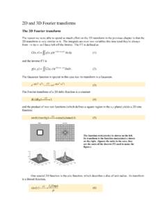
2D and 3D Fourier transforms - Yale University

cryoemprinciples.yale.edu

The discrete Fourier transform The Fourier transform is defined as an integral over all of space. How could we evaluate this on a computer? We will have to take a finite number of discrete samples both in the real (x,y) space and in the (u,v) frequency space. Let’s first do this in one dimension, and we’ll model discrete samples by multiplying

  Discrete

Discrete-Time Signals and Systems - Pearson

www.pearsonhighered.com

The unit sample sequence plays the same role for discrete-time signals and systems that the unit impulse function (Dirac delta function) does for continuous-time signals and systems. For convenience, we often refer to the unit sample sequence as a discrete-time impulse or simply as an impulse. It is important to note that a discrete-time impulse

  Discrete

Lecture 13 Linear dynamical systems with inputs & outputs

see.stanford.edu

Interpretations write x˙ = Ax+b1u1 +···+bmum, where B = [b1 ··· bm] • state derivative is sum of autonomous term (Ax) and one term per input (biui) • each input ui gives another degree of freedom for x˙ (assuming columns of B independent) write x˙ = Ax+Bu as x˙i = ˜aT i x+˜bT i u, where ˜aT i, ˜bT i are the rows of A, B • ith state derivative is linear function of state x ...

  Input

Think DSP - Green Tea Press

greenteapress.com

Think DSP Digital Signal Processing in Python Version 1.1.1 Allen B. Downey Green Tea Press Needham, Massachusetts

  Think, Think dsp

Related search queries