Constrained Optimization Using Lagrange Multipliers

1 Constrained Optimization Using Lagrange MultipliersCEE 201L. Uncertainty, Design, and OptimizationDepartment of Civil and Environmental EngineeringDuke UniversityHenri P. Gavin and Jeffrey T. ScruggsSpring 2020In optimal design problems, values for a set ofndesign variables, (x1,x2, xn), areto be found that minimize a scalar-valued objective function of the design variables, suchthat a set ofminequality constraints, are satisfied. Constrained Optimization problems aregenerally expressed asminx1,x2, ,xnJ=f(x1,x2, ,xn)such thatg1(x1,x2, ,xn) 0g2(x1,x2, ,xn) (x1,x2, ,xn) 0(1)If the objective function is quadratic in the design variables and the constraint equations arelinearly independent, the Optimization problem has a unique the simplest Constrained minimization problem:minx12kx2wherek >0such thatx b .(2)This problem has a single design variable, the objective function is quadratic (J=12kx2),there is a single constraint inequality, and it is linear inx(g(x) =b x).

2 Ifg >0, theconstraint equation constrains the optimum and the optimal solution,x , is given byx = 0, the constraint equation does not constrain the optimum and the optimal solutionis given byx = 0. Not all Optimization problems are so easy; most Optimization methodsrequire more advanced methods. The methods of Lagrange Multipliers is one such method,and will be applied to this simple multiplier methods involve the modification of the objective function throughthe addition of terms that describe the constraints. The objective functionJ=f(x) isaugmentedby the constraint equations through a set of non-negative multiplicativeLagrangemultipliers, j 0. The augmented objective function,JA(x), is a function of thendesignvariables andmLagrange Multipliers ,JA(x1,x2, ,xn, 1, 2, , m) =f(x1,x2, ,xn) +m j=1 jgj(x1,x2, ,xn)(3)For the problem of equation (2),n= 1 andm= 1, soJA(x, ) =12kx2+ (b x) =12kx2 x+ b(4)The Lagrange multiplier, , serves the purpose of modifying (augmenting) the objectivefunction from one quadratic (12kx2) to another quadratic (12kx2 x+ b) so that theminimum of the modified quadratic satisfies the constraint (x b).

3 2 CEE 201L. Uncertainty, Design, and Optimization Duke Spring 2020 Gavin and ScruggsCase 1:b= 1 Ifb= 1 then the minimum of12kx2is Constrained by the inequalityx b, and theoptimal value of should minimizeJA(x, ) atx=b. Figure 1(a) plotsJA(x, ) for a fewnon-negative values of and Figure 1(b) plots contours ofJA(x, ). cost, JA(x)design variable, x = 01233 =4b=1(a) multiplier, design variable, x(b)* variable, multiplier, (x, ) =12kx2 x+ bforb= 1andk= 2.(x , ) = (1,2)CCBY-NC-NDHPG, JTS July 10, 2020 Constrained Optimization Using Lagrange Multipliers3 Figure 1 shows that: JA(x, ) is independent of atx=b, JA(x, ) is minimized atx =bfor = 2, the surfaceJA(x, ) is a saddle shape, the point (x , ) = (1,2) is a saddle point, JA(x , ) JA(x , ) JA(x, ), minxJA(x, ) = max JA(x , ) =JA(x , )Saddle points have no slope. JA(x, ) x x=x = = 0(5a) JA(x, ) x=x = = 0(5b)(5c)For this problem, JA(x, ) x x=x = = 0 kx = 0 =kx (6a) JA(x, ) x=x = = 0 x +b= 0 x =b(6b)This example has a physical interpretation.

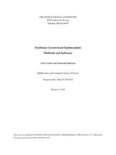
4 The objective functionJ=12kx2representsthe potential energy in a spring. The minimum potential energy in a spring corresponds toa stretch of zero (x = 0). The Constrained problem:minx12kx2such thatx 1means minimize the potential energy in the spring such that the stretch in the spring isgreater than or equal to 1. The solution to this problem is to set the stretch in the springequal to the smallest allowable value (x = 1). Theforceapplied to the spring in order toachieve this objective isf=kx . This forceistheLagrange multiplierfor this problem,( =kx ).The Lagrange multiplier is the force required to enforce the , JTS July 10, 20204 CEE 201L. Uncertainty, Design, and Optimization Duke Spring 2020 Gavin and ScruggsCase 2:b= 1 Ifb= 1 then the minimum of12kx2is notconstrained by the inequalityx b. Thederivation above would givex = 1, with = k. The negative value of indicatesthat the constraint does not affect the optimal solution, and should therefore be set tozero.

5 Setting = 0,JA(x, ) is minimized atx = 0. Figure 2(a) plotsJA(x, ) for a fewnegative values of and Figure 2(b) plots contours ofJA(x, ). cost, JA(x)design variable, x = 0-1-2-3 =-4b=-1(a) multiplier, design variable, x(b)* variable, multiplier, (x, ) =12kx2 x+ bforb= 1andk= 2.(x , ) = (0,0)CCBY-NC-NDHPG, JTS July 10, 2020 Constrained Optimization Using Lagrange Multipliers5 Figure 2 shows that: JA(x, ) is independent of atx=b, the saddle point ofJA(x, ) occurs at a negative value of , so JA/ 6= 0 for any 0. The constraintx 1 does not affect the solution, and is called anon-bindingor aninactiveconstraint. The Lagrange Multipliers associated with non-binding inequality constraints are nega-tive. If a Lagrange multiplier corresponding to an inequality constraint has a negative valueat the saddle point, it is set to zero, thereby removing the inactive constraint from thecalculation of the augmented objective summary, if the inequalityg(x) 0 constrains the minimum off(x) then theoptimum point of the augmented objectiveJA(x, ) =f(x)+ g(x) is minimized with respecttoxand maximized with respect to.

6 The Optimization problem of equation (1) may bewritten in terms of the augmented objective function (equation (3)),max 1, 2, , mminx1,x2, ,xnJA(x1,x2, ,xn, 1, 2, , m)such that j 0 j(7)The necessary conditions for optimality are: JA xk xi=x i j= j= 0(8a) JA k xi=x i j= j= 0(8b) j 0(8c)These equations define the relations used to derive expressions for, or compute values of, theoptimal design variablesx i. Lagrange Multipliers for inequality constraints,gj(x1, ,xn) 0,are non-negative. If an inequalitygj(x1, ,xn) 0 constrains the optimum point, the cor-responding Lagrange multiplier, j, is positive. If an inequalitygj(x1, ,xn) 0 does notconstrain the optimum point, the corresponding Lagrange multiplier, j, is set to , JTS July 10, 20206 CEE 201L. Uncertainty, Design, and Optimization Duke Spring 2020 Gavin and ScruggsSensitivity to Changes in the Constraints and Redundant ConstraintsOnce a Constrained Optimization problem has been solved, it is sometimes useful toconsider how changes in each constraint would affect the optimized cost.

7 If the minimumoff(x) (wherex= (x1, ,xn)) is Constrained by the inequalitygj(x) 0, then at theoptimum pointx ,gj(x ) = 0 and j>0. Likewise, if another constraintgk(x ) does notconstrain the minimum, thengk(x )<0 and k= 0. A small change in thej-th constraint,fromgjtogj+ gj, changes the Constrained objective function fromf(x ) tof(x ) + j , since thek-th constraintgk(x ) does not affect the solution, neither will a smallchange togk, k= 0. In other words, a small change in thej-th constraint, gj, correspondsto a proportional change in the optimized cost, f(x ), and the constant of proportionalityis the Lagrange multiplier of the optimized solution, j. f(x ) =m j=1 j gj(9)The value of the Lagrange multiplier is the sensitivity of the Constrained objective to (small)changes in the constraint g. If j>0 then the inequalitygj(x) 0 constrains the optimumpoint and a small increase of the constraintgj(x )increasesthe cost.

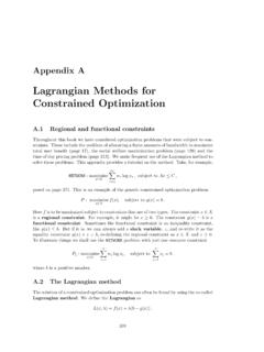
8 If j<0 thengj(x )<0 and does not constrain the solution. A small change of this constraint shouldnot affect the cost. So if a Lagrange multiplier associated with an inequality constraintgj(x ) 0 is computed as a negative value, it is subsequently set to zero. Such constraintsare callednon-bindingorinactiveconstraints. xf(x)g(x)xnot okf(x) >0 f = g(x)+ g g x*x*g(x)not okokok <0 =0 = 0f g(x)+ g Figure : The optimum point is Constrained by the conditiong(x ) 0. A small increaseof the constraint fromgtog+ gincreasesthe cost fromf(x )tof(x )+ g. ( >0) Right:The constraint is negative at the minimum off(x), so the optimum point is not constrainedby the conditiong(x ) 0. A small increase of the constraint function fromgtog+ gdoesnot affect the optimum solution. If this constraint were anequalityconstraint,g(x) = 0, thenthe Lagrange multiplier would be negative and an increase of the constraint woulddecreasethecost fromftof+ g( <0).

9 The previous examples consider the minimization of a simple quadratic with a singleinequality constraint. By expanding this example to two inequality constraints we can seeagain how Lagrange Multipliers indicate whether or not the associated constraint boundsCCBY-NC-NDHPG, JTS July 10, 2020 Constrained Optimization Using Lagrange Multipliers7the optimal solution. Consider the minimization problemminx12kx2such thatx bx cwherek >0and0< b < c(10) xf(x)bnot okokx*=cFigure off(x) =12kx2such thatx bandx cwith0< b < c. Feasiblesolutions forxare greater-or-equal than with the method of Lagrange multipliersJA(x1 1, 2) =12kx2+ 1(b x) + 2(c x)(11)Where the constraints (b x) and (c x) are satisfied if they arenegative-valued. Thederivatives of the augmented objective function are JA(x, 1, 2) x x=x 1= 1 2= 2= 0 kx 1 2= 0(12a) JA(x, 1, 2) 1 x=x 1= 1 2= 2= 0 x +b= 0(12b) JA(x, 1, 2) 2 x=x 1= 1 2= 2= 0 x +c= 0(12c)These three equations are linear inx , 1, and 2.

10 K 1 1 100 100 x 1 2 = 0 b c (13)Clearly, ifb6=cthenxcan not equal bothbandc, and equations (12b) and (12c) cannot both be satisfied. In such cases, we proceed by selecting a subset of the constraints,and evaluating the resulting solutions. So doing, the solutionx =bminimizes12kx2suchthatx bwith a Lagrange multiplier 1=kb. Butx =bdoes not satisfy the inequalityx c. The solutionx =cminimizes12kx2. such that both inequalities hold and withwith a Lagrange multiplier 2=kc. Note that for this quadratic objective, the constraintwith the larger Lagrange multiplier is the active constraint and that the other constraint , JTS July 10, 20208 CEE 201L. Uncertainty, Design, and Optimization Duke Spring 2020 Gavin and ScruggsMultivariable Quadratic ProgrammingQuadratic Optimization problems with a single design variable and a single linear in-equality constraint are easy enough. In problems with many design variables (n 1) andmany inequality constraints (m 1), determining which inequality constraints are enforcedat the optimum point can be difficult.