Correlation in Random Variables

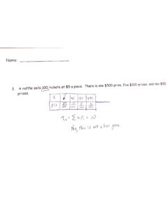
1 Correlation in Random VariablesLecture 11 Spring 2002 Correlation in Random VariablesSuppose that an experimentproduces two Random vari-ables, about the relationship be-tween them?One of the best ways to visu-alize the possible relationshipis to plot the (X, Y)pairthatis produced by several trials ofthe experiment. An exampleof correlated samples is shownat the rightLecture 111 Joint Density FunctionThe joint behavior ofXandYis fully captured in the joint probabilitydistribution. For a continuous distributionE[XmYn]= xmynfXY(x, y)dxdyFor discrete distributionsE[XmYn]= x Sx y SyxmynP(x, y)Lecture 112 Covariance FunctionThe covariance function is a number that measures the commonvariation is defined ascov(X, Y)=E[(X E[X])(Y E[Y])]=E[XY] E[X]E[Y]The covariance is determined by the difference inE[XY]andE[X]E[Y].IfXandYwere statistically independent thenE[XY] would equalE[X]E[Y] and the covariance would be covariance of a Random variable with itself is equal to its [X, X]=E[(X E[X])2]=var[X]Lecture 113 Correlation CoefficientThe covariance can be normalized to produce what is known as thecorrelation coefficient.

2 =cov(X,Y) var(X)var(Y)The Correlation coefficient is bounded by 1 will havevalue = 0 when the covariance is zero and value = 1 whenXandYare perfectly correlated or 114 Autocorrelation FunctionThe autocorrelation function is very similar to the covariance func-tion. It is defined asR(X, Y)=E[XY]=cov(X, Y)+E[X]E[Y]It retains the mean values in the calculation of the value. Therandom Variables areorthogonalifR(X, Y)= 115 Normal DistributionfXY(x, y)=12 x y 1 2exp x x x 2 2 x x x y y y + y y y 22(1 2) Lecture 116 Normal DistributionThe orientation of the elliptical contours is along the liney=xif >0 and along the liney= xif < contours are a circle,and the Variables are uncorrelated, if = center of the ellipseis( x, y).Lecture 117 Linear EstimationThe task is to construct a rule for the prediction YofYbased onan observation the Random Variables are correlated then this should yield a betterresult, on the average, than just guessing.

3 We are encouraged toselect a linear rule when we note that the sample points tend to fallabout a sloping line. Y=aX+bwhereaandbare parameters to be chosen to provide the bestresults. We would expectato correspond to the slope andbto 118 Minimize Prediction ErrorTo find a means of calculating the coefficients from a set of samplepoints, construct the predictor error =E[(Y Y)2]We want to chooseaandbto minimize .Therefore, compute theappropriate derivatives and set them to zero. a= 2E[(Y Y) Y a]=0 b= 2E[(Y Y) Y b]=0 These can be solved foraandbin terms of the expected expected values can be themselves estimated from the 119 Prediction Error EquationsThe above conditions onaandbare equivalent toE[(Y Y)X]=0E[Y Y]=0 The prediction errorY Ymust be orthogonal toXand the expectedprediction error must be Y=aX+bleads to a pair of equations to be [(Y aX b)X]=E[XY] aE[X2] bE[X]=0E[Y aX b]=E[Y] aE[X] b=0 E[X2]E[X]E[X]1 ab = E[XY]E[Y] Lecture 1110 Prediction Errora=cov(X,Y)var(X)b=E[Y] cov(X,Y)var(X)E[X]The prediction error with these parameter values is =(1 2)var(Y)

4 When the Correlation coefficient = 1 the error is zero, meaningthat perfect prediction can be = 0 the variance in the prediction is as large as the variationinY,and the predictor is of no help at intermediate values of , whether positive or negative, the pre-dictor reduces the 1111 Linear Predictor ProgramThe the coefficients [a, b] as well as thecovariance matrixCand the Correlation coefficient, . The covari-ance matrix isC= var[X]cov[X, Y]cov[X, Y]var[Y] Usage example:N=100X=Randomn(seed,N)Z=Randomn( seed,N)Y=2*X-1+ *Zp=lp(X,Y,c,rho)print, Predictor Coefficients= ,pprint, Covariance matrix print,cprint, Correlation Coefficient= ,rhoLecture 1112 Program lpfunction lp,X,Y,c,rho,mux,muy;Compute the linear predictor coefficients such that;Yhat=aX+b is the minimum mse estimate of Y based on X.;Shorten the X and Y vectors to the length of the (X) < n_elements(Y)X=(X[0:n-1])[*]Y=(Y[0:n-1]) [*];Compute the mean value of (X)/nmuy=total(Y)/nContinued on next pageLecture 1113 Program lp (continued);Compute the covariance [[X-mux],[Y-muy]]C=V##transpose(V)/(n-1) ;Compute the predictor coefficient and [0,1]/c[0,0]b=muy-a*mux;Compute the Correlation coefficientrho=c[0,1]/sqrt(c[0,0]*c[1,1] )Return,[a,b]ENDL ecture 1114 ExamplePredictor Coefficients= Coefficient= 1115 IDL Regress FunctionIDL provides a number of routines for the analysis of data.

5 Thefunction REGRESS does multiple linear the predictor coefficientaand constantbbya=regress(X,Y,Const=b)print,[ a,b] 1116 New ConceptIntroduction to Random ProcessesToday we will just introduce the basic 1117 Random ProcessesLecture 1118 Random Process A Random variable is a functionX(e) that maps the set of ex-periment outcomes to the set of numbers. Arandom processis a rule that maps every outcomeeof anexperiment to afunctionX(t, e). A Random process is usually conceived of as a function of time,but there is no reason to not consider Random processes that arefunctions of other independent Variables , such as spatial coordi-nates. The functionX(u, v, e) would be a function whose value de-pended on the location (u, v) and the outcomee,and could beused in representing Random variations in an 1119 Random Process The domain ofeis the set of outcomes of the experiment.

6 Weassume that a probability distribution is known for this set. The domain oftis a set,T,of real numbers. IfTis the real axis thenX(t, e)isacontinuous-timerandomprocess IfTis the set of integers thenX(t, e)isadiscrete-timerandomprocess We will often suppress the display of the variableeand writeX(t)for a continuous-time RP andX[n]orXnfor a discrete-time 1120 Random Process A RP is a family of functions,X(t, e).Imagine a giant strip chartrecording in which each pen is identified with a of functions is traditionally called anensemble. A single functionX(t, ek) is selected by the isjust a time function that we could callXk(t).Different outcomesgive us different time functions. Iftis fixed, sayt=t1,thenX(t1,e) is a Random variable. Itsvalue depends on the outcomee. If bothtandeare given thenX(t, e) is just a 1121 Moments and AveragesX(t1,e) is a Random variable that represents the set of samples acrossthe ensemble at timet1If it has a probability density functionfX(x;t1) then the momentsaremn(t1)=E[Xn(t1)] = xnfX(x;t1)dxThe notationfX(x;t1) may be necessary because the probabilitydensity may depend upon the time the samples are mean value is X=m1,which may be a function of central moments areE[(X(t1) X(t1))n]= (x X(t1))nfX(x;t1)dxLecture 1122 Pairs of SamplesThe numbersX(t1,e)andX(t2,e) are samples from the same timefunction at different are a pair of Random Variables (X1,X2).

7 They have a joint probability density functionf(x1,x2;t1,t2).From the joint density function one can compute the marginal den-sities, conditional probabilities and other quantities that may be 1123