CS229LectureNotes - Stanford University

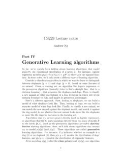
1 CS229 Lecture Notes Andrew Ng (updates by Tengyu Ma). Supervised learning Let's start by talking about a few examples of supervised learning problems. Suppose we have a dataset giving the living areas and prices of 47 houses from Portland, Oregon: Living area (feet2 ) Price (1000$s). 2104 400. 1600 330. 2400 369. 1416 232. 3000 540.. We can plot this data: housing prices 1000. 900. 800. 700. 600. price (in $1000). 500. 400. 300. 200. 100. 0. 500 1000 1500 2000 2500 3000 3500 4000 4500 5000. square feet 1. 2. Given data like this, how can we learn to predict the prices of other houses in Portland, as a function of the size of their living areas? To establish notation for future use, we'll use x(i) to denote the input . variables (living area in this example), also called input features, and y (i). to denote the output or target variable that we are trying to predict (price).

2 A pair (x(i) , y (i) ) is called a training example, and the dataset that we'll be using to learn a list of n training examples {(x(i) , y (i) ); i =. 1, .. , n} is called a training set. Note that the superscript (i) in the notation is simply an index into the training set, and has nothing to do with exponentiation. We will also use X denote the space of input values, and Y. the space of output values. In this example, X = Y = R. To describe the supervised learning problem slightly more formally, our goal is, given a training set, to learn a function h : X 7 Y so that h(x) is a good predictor for the corresponding value of y. For historical reasons, this function h is called a hypothesis. Seen pictorially, the process is therefore like this: Training set Learning algorithm x h predicted y (living area of (predicted price). house.) of house). When the target variable that we're trying to predict is continuous, such as in our housing example, we call the learning problem a regression prob- lem.

3 When y can take on only a small number of discrete values (such as if, given the living area, we wanted to predict if a dwelling is a house or an apartment, say), we call it a classification problem. 3. Part I. Linear regression To make our housing example more interesting, let's consider a slightly richer dataset in which we also know the number of bedrooms in each house: Living area (feet2 ) #bedrooms Price (1000$s). 2104 3 400. 1600 3 330. 2400 3 369. 1416 2 232. 3000 4 540.. (i). Here, the x's are two-dimensional vectors in R2 . For instance, x1 is the (i). living area of the i-th house in the training set, and x2 is its number of bedrooms. (In general, when designing a learning problem, it will be up to you to decide what features to choose, so if you are out in Portland gathering housing data, you might also decide to include other features such as whether each house has a fireplace, the number of bathrooms, and so on.)

4 We'll say more about feature selection later, but for now let's take the features as given.). To perform supervised learning, we must decide how we're going to rep- resent functions/hypotheses h in a computer. As an initial choice, let's say we decide to approximate y as a linear function of x: h (x) = 0 + 1 x1 + 2 x2. Here, the i 's are the parameters (also called weights) parameterizing the space of linear functions mapping from X to Y. When there is no risk of confusion, we will drop the subscript in h (x), and write it more simply as h(x). To simplify our notation, we also introduce the convention of letting x0 = 1 (this is the intercept term), so that d X. h(x) = i xi = T x, i=0. where on the right-hand side above we are viewing and x both as vectors, and here d is the number of input variables (not counting x0 ). 4. Now, given a training set, how do we pick, or learn, the parameters ?

5 One reasonable method seems to be to make h(x) close to y, at least for the training examples we have. To formalize this, we will define a function that measures, for each value of the 's, how close the h(x(i) )'s are to the corresponding y (i) 's. We define the cost function: n 1X. J( ) = (h (x(i) ) y (i) )2 . 2 i=1. If you've seen linear regression before, you may recognize this as the familiar least-squares cost function that gives rise to the ordinary least squares regression model . Whether or not you have seen it previously, let's keep going, and we'll eventually show this to be a special case of a much broader family of algorithms. 1 LMS algorithm We want to choose so as to minimize J( ). To do so, let's use a search algorithm that starts with some initial guess for , and that repeatedly changes to make J( ) smaller, until hopefully we converge to a value of that minimizes J( ).

6 Specifically, let's consider the gradient descent algorithm, which starts with some initial , and repeatedly performs the update: . j := j J( ). j (This update is simultaneously performed for all values of j = 0, .. , d.). Here, is called the learning rate. This is a very natural algorithm that repeatedly takes a step in the direction of steepest decrease of J. In order to implement this algorithm, we have to work out what is the partial derivative term on the right hand side. Let's first work it out for the case of if we have only one training example (x, y), so that we can neglect the sum in the definition of J. We have: 1. J( ) = (h (x) y)2. j j 2. 1 . = 2 (h (x) y) (h (x) y). 2 j d ! X. = (h (x) y) i x i y j i=0. = (h (x) y) xj 5. For a single training example, this gives the update rule:1. (i). j := j + y (i) h (x(i) ) xj . The rule is called the LMS update rule (LMS stands for least mean squares ), and is also known as the Widrow-Hoff learning rule.

7 This rule has several properties that seem natural and intuitive. For instance, the magnitude of the update is proportional to the error term (y (i) h (x(i) )); thus, for in- stance, if we are encountering a training example on which our prediction nearly matches the actual value of y (i) , then we find that there is little need to change the parameters; in contrast, a larger change to the parameters will be made if our prediction h (x(i) ) has a large error ( , if it is very far from y (i) ). We'd derived the LMS rule for when there was only a single training example. There are two ways to modify this method for a training set of more than one example. The first is replace it with the following algorithm: Repeat until convergence {. n X (i). j := j + y (i) h (x(i) ) xj , (for every j) (1). i=1. }. By grouping the updates of the coordinates into an update of the vector , we can rewrite update (1) in a slightly more succinct way: n X.

8 Y (i) h (x(i) ) x(i).. := + . i=1. The reader can easily verify that the quantity in the summation in the update rule above is just J( )/ j (for the original definition of J). So, this is simply gradient descent on the original cost function J. This method looks at every example in the entire training set on every step, and is called batch gradient descent. Note that, while gradient descent can be susceptible to local minima in general, the optimization problem we have posed here 1. We use the notation a := b to denote an operation (in a computer program) in which we set the value of a variable a to be equal to the value of b. In other words, this operation overwrites a with the value of b. In contrast, we will write a = b when we are asserting a statement of fact, that the value of a is equal to the value of b. 6. for linear regression has only one global, and no other local, optima; thus gradient descent always converges (assuming the learning rate is not too large) to the global minimum.

9 Indeed, J is a convex quadratic function. Here is an example of gradient descent as it is run to minimize a quadratic function. 50. 45. 40. 35. 30. 25. 20. 15. 10. 5. 5 10 15 20 25 30 35 40 45 50. The ellipses shown above are the contours of a quadratic function. Also shown is the trajectory taken by gradient descent, which was initialized at (48,30). The x's in the figure (joined by straight lines) mark the successive values of that gradient descent went through. When we run batch gradient descent to fit on our previous dataset, to learn to predict housing price as a function of living area, we obtain 0 = , 1 = If we plot h (x) as a function of x (area), along with the training data, we obtain the following figure: housing prices 1000. 900. 800. 700. 600. price (in $1000). 500. 400. 300. 200. 100. 0. 500 1000 1500 2000 2500 3000 3500 4000 4500 5000. square feet 7. If the number of bedrooms were included as one of the input features as well, we get 0 = , 1 = , 2 = The above results were obtained with batch gradient descent.

10 There is an alternative to batch gradient descent that also works very well. Consider the following algorithm: Loop {. for i = 1 to n, {. (i). j := j + y (i) h (x(i) ) xj , (for every j) (2). }. }. By grouping the updates of the coordinates into an update of the vector , we can rewrite update (2) in a slightly more succinct way: := + y (i) h (x(i) ) x(i).. In this algorithm, we repeatedly run through the training set, and each time we encounter a training example, we update the parameters according to the gradient of the error with respect to that single training example only. This algorithm is called stochastic gradient descent (also incremental gradient descent). Whereas batch gradient descent has to scan through the entire training set before taking a single step a costly operation if n is large stochastic gradient descent can start making progress right away, and continues to make progress with each example it looks at.