Transcription of DESCRIBING AND USING DATA - …
1 COLLECTING data / 9 CHAPTER TWO DESCRIBING AND USING data data is the foundation from which all scientific inferences are made. The observations we make on our sample patients allow us to answer hypotheses about the population-at-large. The collection of data is one of the more tedious aspects of medical research and biostatistics. It is also one of the most crucial aspects if meaningful and accurate conclusions are to be drawn from the data . No amount of statistical manipulation can overcome data which is either not collected to begin with or is collected improperly.
2 It is therefore essential to consider the types of data that will be necessary to answer the proposed research hypotheses before data collection begins to ensure that the correct types of data will be available for analysis later. TYPES OF VARIABLES There are many different types of data each of which requires specific statistical tests for correct analysis . The characteristics of interest in any study are called variables. Study variables may include age, sex, height, weight, blood pressure, cardiac output, survival, or any of a multitude of other characteristics. There are two major types of variables: discrete (or categorical) and continuous (Figure 2-1).
3 data Variables Discrete (or Categorical) Continuous - age - heart rate Binary (or Nominal) Ordinal - systolic blood pressure - yes or no - excellent, good, fair, poor - cardiac output - male vs female - Stage I, II, III, IV - live vs die - Duke s A, B, C, D Figure 2-1: Types of data Variables Discrete or categorical variables are those which can only assume certain fixed or integer values. Discrete variables can be further divided into two categories: binary (or nominal) and ordinal. Binary or nominal variables are those whose values are either yes or no.
4 Examples include sex (male vs female), survival (live vs die), disease (cancer vs no cancer), or outcome (extubated vs reintubated). Ordinal variables are those whose values fall into categories, but are not limited to only two results. Examples of ordinal variables include outcome (excellent, good, fair, poor, no change) or disease stages (such as tumor staging classifications). Continuous variables are those which can assume an infinite range of values. Age, heart rate, systolic blood pressure, and cardiac output are examples of continuous variables. It is important to make a distinction between discrete and continuous variables as each requires a different set of statistical tests for proper analysis .
5 Variables can be further categorized as being either dependent or independent. Dependent variables are those whose value depends on that of another factor which is termed an independent variable. An example of a dependent variable is mean arterial blood pressure which is calculated from the systolic and diastolic blood pressures (both of which are examples of independent variables). A confounding variable is one which is closely associated with the outcome of interest (the dependent variable) such that it is unclear whether an observation is a reflection of the relationship between the confounding and dependent variables or between the independent and dependent variables.
6 Consider a study that addresses whether therapy with H2 blockers (the independent variable) influences the occurrence of peptic ulcer disease (the dependent variable). If fewer ulcers are seen in patients receiving H2 blockers, we might conclude that H2 blockers decrease the incidence of peptic ulcer disease. If the study patients were also receiving antacid therapy (a potential confounding variable), however, our conclusions might be in error as the decrease in ulcer incidence could be due to the H2 blockers or the antacids or a combination of the two. There is an infinite list of potential confounding variables in any study and the goal of study design is to minimize the potential effect of such 10 / A PRACTICAL GUIDE TO BIOSTATISTICS variables on data analysis and study conclusions.
7 It is important to account for confounding variables in the design and statistical analysis of studies in order to avoid incorrect conclusions. The most effective way to accomplish this is to perform a randomized study in which the effect of confounding variables is theoretically be distributed equally between the study and control groups (see Chapter Nine). Observations collected on a study sample will tend to be grouped in some form of pattern. Only rarely will all of our observations be identical. In most situations, they will all be slightly different due to natural biologic variability.
8 They will, however, tend to be grouped towards a middle or central point. If our sample closely approximates the population of interest, observations from the sample and the population should be centered around the same point. One way to confirm that our sample data is representative of the population is to plot or graph the observations. This results in a frequency distribution or histogram such as that below (Figure 2-2) where each x indicates a patient with a post-operative myocardial infarction. x x frequency of x x x post-operative x x x myocardial x x x x x infarction x x x x x x x 1 2 3 4 5 6 7 post-operative days Figure 2-2.
9 Frequency histogram From this histogram it is clear that the observations are more or less centered around the 3rd day and appear to be equally distributed on either side. We can conclude from this graph that most post-operative myocardial infarctions occur on the 3rd post-operative day, but can occur with less frequency on any of the first 7 days following surgery. Such a symmetric pattern (which takes the appearance of a bell-shaped curve) is called a normal, gaussian, or z distribution (after the German mathematician, Johann Gauss, who first described it) and is characterized by the distribution having the same slope on both sides of the center of the data (Figure 2-3a).
10 Not all observations are symmetrically distributed, however. If the observations fall predominantly to one side or the other and are not evenly distributed around the center of the data (as in a normal distribution), the data are said to be skewed or non-normally distributed (Figure 2-3b). Just as the type of variable determines the correct statistical test to be used, the type of distribution determines whether a statistical test for normally or non-normally distributed data must be used. a) normal (z) distribution b) non-normal distribution Figure 2-3: Types of distributions data which are skewed or non-normally distributed can present problems with statistical analysis .