Transcription of Determination of Trace Elements in Steels and …
1 Determination of Trace Elements in Steels and alloys using the Thermo Scientific iCAP 7400 ICP-OESAPPLICATION NOTE 43146 AuthorsSanja Asendorf, Application Specialist, Thermo Fisher Scientific, Bremen, GermanyKeywordsAlloy, Microwave digestion, SteelIntroductionSteels and iron alloys are among the most flexible and widely used metals in industry. They can be formed, drawn, cast or turned to shape with a wide range of finishes such as polishing, plating or simply painting. This flexibility means that they have found a wide range of applications from constructional use to surgical implements.
2 The properties of the steel can be enhanced or changed to suit the application depending on the constituent Elements . For example, addition of nickel, chromium and manganese give corrosion resistance whilst the addition of carbon improves the hardness of a cutting edge. In order to maintain a consistent quality of steel, it is necessary to determine the Trace elemental composition very accurately. Inductively Coupled Plasma Optical Emission Spectrometry (ICP-OES) is an ideal technique for this analysis since the wide linear dynamic range allows for the Determination of minor and Trace Elements simultaneously, without the need for additional dilution or pre-concentration techniques, resulting in time and cost efficient sample preparation and rapid, precise and accurate Determination of minor and Trace Elements in Steels and iron alloys is analytically demanding, but of great commercial significance.
3 This note demonstrates that closed vessel microwave digestion, followed by analysis using the Thermo Scientific iCAP 7000 Plus Series ICP-OES, provides a cost effective , samples are prepared by dissolution using mixed acids in an open beaker1. However, this approach is time consuming and can result in the partial loss of Elements , particularly the more volatile Elements . In order to aid the digestion of samples, closed vessel dissolution is increasingly used, as it allows for the use of higher temperatures and pressures. The use of microwave power, rather than a conventional oven or hotplate, further increases the efficiency of the digestion and shortens the required Thermo Scientific iCAP 7400 ICP-OES Radial fitted with a standard sample introduction kit was used for this analysis.
4 The radial plasma instrument was selected for its robust matrix handling abilities, in order to minimize interferences. The high-resolution echelle optics and Charge Injection Device (CID) detector are especially well suited to this type of application where Trace amounts of an element must be detected in the presence of matrix and standard preparationTwo samples were obtained: 1) ECISS Euronorm ZRM 467-3 (Rohesian) and 2) GBW 01323 (steel, China). Both were supplied by MBH Analytical Ltd. UK. The samples were digested in a Milestone ETHOS EZ microwave digestion system.
5 Masses of g of the samples (reference materials) were weighed into digestion vessels and 10 ml of concentrated hydrochloric acid (34 37% TraceMetal grade, Fisher Scientific, Loughborough, UK) and 2 ml of concentrated nitric acid ( 68% TraceMetal grade, Fisher Scientific, Loughborough, UK) were added. The vessels were closed and fitted into the rotor and digested at 180 C for 20 minutes. When the microwave program was finished, the digestion vessels were left to cool and the contents made up to 100 g with ultra-pure deionized water. All of the samples produced clear solutions after digestion although a small quantity of white material, assumed to be silica, was observed in several of the solutions.
6 The sample was filtered to remove these particles prior to analysis. Multi-element working standards were prepared from 1000 mg L-1 single element solutions (Fisher Scientific, Loughborough, UK) by dilution with mixed acid blank solution. Concentrations used for the analysis are given in Table 1. Reagent blanks were prepared by omitting the samples from two 1. Concentration of standards in mg 1 Standard 2Cr 0 2 20 Cu 0 10 20 Mn 0 20 100 Ni 0 1 10 P 0 1 10 Ti 0 5 V 0 2 20 Method development A LabBook was created using the Thermo Scientific Qtegra Intelligent Scientific Data Solution (ISDS) Software.
7 For each element, wavelengths were selected using the intuitive wavelength selection tool of the Qtegra ISDS Software. The wavelengths used for analysis are shown in Table 3, these were selected as they were free from interferences and provided the sensitivity to quantify the Elements of interest in the expected concentration range. Optionally, these steps can be simplified by using the Qtegra ISDS Software Element Finder plug-in. The plasma was ignited and the instrument allowed to warm up for a period of 30 minutes. A standard, sample and blank were analyzed and the subarrays were examined to check for any background shifts or spectral overlaps.
8 Sample introduction and plasma conditions were optimized to give maximal signal-to-background ratios (SBRs) and these optimized parameters are shown in Table 2. Optimal sample introduction and plasma ViewRadialPump Tubing (Standard Pump)Sample Tygon orange/whiteDrain Tygon white/whitePump Speed 50 rpm Spray Chamber Glass cyclonic Center Tube mm Nebulizer Glass concentric Nebulizer Gas Flow L min-1 Auxiliary Gas Flow L min-1 Coolant Gas Flow 12 L min-1RF Power 1150 W Exposure Time UV 15 s, Vis 10 s Working standards were used to produce element calibration fits in Qtegra ISDS Software, these calibration lines were checked to ensure an accurate fit and correlation coefficients (R2)
9 Of better than were obtained for all Elements examined. For analysis where the element concentrations exceeded the standard s value, a dilution (matrix matched for acid content) was 3. Method detection limit (MDL) for different analyte wavelengths in g 4. Elemental composition of measured samples compared with the certified value in %.Element and wavelength (nm)MDLCr C u 3 2 7. 3 9 6 Mn Ni P 6 Ti V 4 Element ZRM 476-3 expectedZRM 476-3 measuredGBW 01323 expectedGBW 01323 measuredCr Cu Mn 0 9 Ni 0.
10 161 P 0 . 011 Ti V 0 .14 8 ResultsMethod detection limits (Table 3) were calculated by calibrating the instrument with the standards stipulated in the method and reanalyzing the sample blank. The standard deviation of ten replicates of the blank was multiplied by 3 to give a 3 detection limit in g L-1 in solution, which is shown in Table digested samples, detailed above, were then analyzed and the results compared to their certified values (see Table 4). The results show good agreement between the measured and specified elemental concentrations for both Research Use Only.