Transcription of Fermi’s Golden Rule - USTC
1 Fermi s Golden RuleEmmanuel N. : 198 AbstractWe present a proof of Fermi s Golden rule from an educational perspectivewithout compromising IntroductionFermi s Golden Rule (also referred to as, theGolden Rule of time-dependentperturbation theory) is an equation for calculating transition rates. Theresult is obtained by applying the time-dependent perturbation theory to asystem that undergoes a transition from an initial state|i to a final state|f that is part of a continuum of following sections provide the calculations and notions involved inderiving the final equation, as well as some concluding remarks (synopsis).2. Time dependent perturbation theoryFor a great deal of problems the time-independent perturbation theory suf-fices. Nevertheless, there are cases in which we want to study how systemsrespond to imposed perturbations and then settle into stationary states afteran interval, in other words, study the transitions induced by a perturbationbetween stationary states of the unperturbed system.
2 In cases like these, weuse time-dependent perturbation theory to calculate, amongst other things,transition assume that the hamiltonian H of the system can be written in theform:H=H0+W(t)(1)where,H0is the hamiltonian of the unperturbed system,W(t) is a perturbation applied to the the unperturbed hamiltonian, the time independent Schr odingerequation is satisfied:H0| n =En| n (2)The wavefunctions| n are related to the time-dependent unperturbedwavefunctions by:| n(t) =| n e iEnt/ h(3)The time dependent Schr odinger equation for the system is:H| (t) = [H0+W(t)]| (t) =i h | (t) t(4)with the state of the system| , at a time t, expressed as a linear combina-tion of the{| n }basis functions:| (t) = ncn(t)| n(t) = ncn(t)| n e iEnt/ h(5)3We insert this relation in (4) and project the result on| n :H0 kck(t)| k e iEkt/ h+W(t) kck(t)| k e iEkt/ h=i h t kck(t)| k e iEkt/ h kck(t)Ek| k e iEkt/ h+ kck(t)W(t)| k e iEkt/ h=i h k ck(t) t| k e iEkt/ h+i h kck(t)| k ( iEk h)e iEkt/ h Encn(t)e iEnt/ h+ kck(t)Wnk(t)e iEkt/ h=i h cn(t) te iEnt/ h+Encn(t)e iEnt/ h kck(t)Wnk(t)e iEkt/ h=i h cn(t) te iEnt/ h cn(t) t=1i h kck(t)Wnk(t)ei nkt(6)where,Wnk= n|W(t)| k , the perturbation matrix element, nk= (En Ek)/ hUp to this point we have made no approximation.
3 The difficulty insolving (6) arises from the fact that the coefficients are expressed in termsof themselves. In order to evaluate the coefficients from (6) we make system is initially in state|i , thus, all of the coefficients at t=0are equal to zero, except forci:cj(t= 0) = perturbation is very weak and applied for a short period of time,such that all of the coefficients remain nearly these in mind, (6) gives us: cn(t) t=1i hci(t)Wni(t)ei nit(7)so for any final state the coefficient will be (cf(t) cf(0) = 0):4cf(t) =1i h t0 Wfi(t )ei fit dt (8)remarksIn order to derive (8) we forced all of the coefficients of the states toremain virtually unchanged, at time t, from the values they initially had(t=0). For that we must pay a price. Equation (8) holds only for perturba-tions that last a very short period of time, that don t have enough timeto significantly alter the state of the , by zeroing out the coefficients of states in (6) we deprived thesystem of any capability of reaching the final state by alternate routes, direct transitions from state|i to|f are have extensively used frases that refer to transitions betweeneigen-statesof the unperturbed hamiltonianH0.
4 Such frases are commonplacein Quantum Mechanics literature1but are also a point of much controversyand discussions. The controversy has to do mainly with the interpretationone gives to the mathematical results of Quantum Mechanics. As an ex-ample of the situation a quotation is given from the very well known andaccepted bookQuantum Mechanics, by L. E. Ballentine[5, p. 351] (whosupports[6] an interpretation for the wavefunction other than theorthodoxinterpretation): When problems of this sort are discussed formally, it is com-mon to speak of the perturbation as causingtransitionsbetweenthe eigenstatesH0. If this means only that the system has ab-sorbed from the perturbing field (or emitted to it) the energydifference h fi= f i, and so has changed its energy, thereis no harm in such language.
5 But if the statement is interpretedto mean that the state has changed from its initial value of| (0) =|i to a final value of| (T) =|f , then it is ..If the state vector| is of the form (5) it is correct to saythat the probability of the energy being fis|cf|2. In the for-mal notation this becomesProb(E= f| ) =| f|2, which is acorrect formula of quantum theory. But it is nonsense to speakof the probability of the state being|f when in fact the state is| . The application of the perturbation changes the state of the system fromthe initial state| i to a final state| f , both of which are eigenstates of1 This language is used by Cohen-Tannoudji, Atkins, Merzbacher [1, 2, 3, 4] and unperturbed hamiltonianH0. The probability of finding the system inthe eigenstate| f is:Pif(t) =| f| (t) |2(9)Using (8) we have:Pif(t) =1 h2 t0ei fit Wfi(t )dt 2(10)3.
6 High frequency harmonic perturbationThe case of an oscillating ( harmonic) perturbation is a most importantone. Once the effects of an oscillating perturbation are known then the gen-eral case can be evaluated since an arbitrary perturbation can be expressedas a superposition of harmonic functions. An example of an oscillating per-turbation is an electromagnetic wave such as a laser define the oscillating perturbation having the form:W(t) = 2 Wcos( t) =W(ei t+e i t)(11)Inserting this in (8) we obtain:cf(t) =Wfii h t0(ei t +e i t )ei fit dt =Wfii h{ei( fi+ )t 1i( fi+ )+ei( fi )t 1i( fi )}(12)Thus, equation (10) becomes:Pif(t) =W2fi h2 ei( fi+ )t 1i( fi+ )+ei( fi )t 1i( fi ) 2(13)At this point we make an approximation assuming that the oscillatingangular frequency of the perturbation has a value near the Bohr angularfrequency of| i and| f , fi: ' fiwhich can also be written:| fi| | fi|With this approximation, the first term in equation (13) becomes negli-gible compared to the second one.
7 This is made obvious from the fact that6the exponential factor (eix=cosx+isinx) cannot become greater than , the prominent term is defined by the denominator. When ' fi(usualy of high frequency fi 1015sec 1) the denominator of the secondterm goes to zero (the situation is reversed when ' fi, so we need notexamine this case separately).The second term (also called the resonant term ) can be written:A =ei( fi )t 1i( fi )=ei( fi )t/2ei( fi )t/2 e i( fi )t/2i( fi )=ei( fi )t/2sin[( fi )t/2]( fi )/2(14)Thus, the probability becomes:Pif(t) =W2fi h2 sin[( fi )t/2]( fi )/2 2(15)and, by introducing the functionF(t, fi):F(t, fi) ={sin[( fi )t/2]( fi )/2}2(16)we obtain:Pif(t) =W2fi h2F(t, fi)(17)remarksAs we can see in the figure (1) the functionF(t, ) has a sharp peakabout the central angular frequency.
8 Do to this behavior we say that F,and thus the probabilityPif(t; ), shows aresonantnature. The distancebetween the first two zeros are defined as the resonance width . The areaunderlined byPif(t; ) at this interval is over 95% of the total area. For we have: '4 t(18)The functionF(t, ) appears in equation (17) with an offset. As a result,the resonant point is located at = fi. The modulus of the resonant termin equation (13),|A |2, behaves in the same manner. In the antiresonantcase,|A+|2, the resonant point is located at = fi. Placing both ofthese functions on the same graph it becomes clear that the part of|A+|27 Figure 1: The functionF(t, ) shows a resonant reaches fiis the diffraction pattern (negligible). In view of this, theresonant approximation is justified when|A+|2and|A |2are far apart:2| fi| (19)and with (18), we obtain:t 1| fi|'1 (20)Another point noteworthy is the behavior of the probability function atresonance.
9 From equation (17) at the resonant frequency we havePif(t; = fi) =W2fi h2t2(21)from which we acquire probability values greater than one for large valuesof t. For this equation to have physical meaning the probabilityPifmust8be less than 1, which we have when:t h|Wfi|(22)and using, (20):1| fi| h|Wfi|(23)which we can read as: the matrix element of the perturbation must be muchsmaller than the energy separation between the initial and final Quantum jumps to the continuumWhen the final state is part of a continuum of states ( when the energybelongs to a continuous part of the spectrum ofH0) we must account forall the states to which the system can jump to. This is done by integratingthe probability as given by equation (17) with thedensity of states (E) asweights:P(t) = {Eacc}Pif(t) (E)dE(24),where{Eacc}denotes all the states that the system can jump to underthe influence of the perturbation.
10 (What we have actually done is create a probability density from the prob-ability equation).The probability function is sharply peaked at = fiand as a resultacts as a delta function in the integral and thus selects the value for thedensity function at = fi. By substituting equation (17) in (24) we have:P(t) = {Eacc}W2fi h2F(t, fi) (E)dE= {Eacc}W2fi h2{sin[( fi )t/2]( fi )/2}2 (E)dEas shown in the figure (2) the range of energies is very narrow and asa result the matrix elementWfiand the density of states (E) can beconsidered as constant:9 Figure 2: The functionF(t, ) acts as a delta (t) =W2fi h2 (Efi) {Eacc}{sin[( fi )t/2]( fi )/2}2dE=W2fi h2 (Efi) {Eacc}{sin[( fi )t/2]( fi )/2}2 hd =W2fi h2 (Efi) h(2t)t2 + sin2xx2dxwhere we substitutedE= h ,x= ( fi )t/2 and used the fact thatfor frequencies far from fithe functionsin2x/x2is negligible so we canextend the limits to infinity.