Forecasting with moving averages - Duke University

1 1 1. Simple moving averages 2. Comparing measures of forecast error between models 3. Simple exponential smoothing 4. Linear exponential smoothing 5. A real example: housing starts revisited 6. Out-of-sample validation 1. SIMPLE moving averages In previous classes we studied two of the simplest models for predicting a model from its own history the mean model and the random walk model. These models represent two extremes as far as time series Forecasting is concerned. The mean model assumes that the best predictor of what will happen tomorrow is the average of everything that has happened up until now. The random walk model assumes that the best predictor of what will happen tomorrow is what happened today, and all previous history can be ignored. Intuitively there is a spectrum of possibilities in between these two extremes.

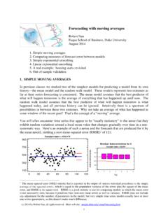
2 Why not take an average of what has happened in some window of the recent past? That s the concept of a moving average . You will often encounter time series that appear to be locally stationary in the sense that they exhibit random variations around a local mean value that changes gradually over time in a non-systematic way. Here s an example of such a series and the forecasts that are produced for it by the mean model, yielding a root-mean-squared error (RMSE)1 of 121: 1 The mean squared error (MSE) statistic that is reported in the output of various statistical procedures is the simple average of the squared errors, which is equal to the population variance of the errors plus the square of the mean error, and RMSE is its square root. RMSE is a good statistic to use for comparing models in which the mean error is not necessarily zero, because it penalizes bias (non-zero mean error) as well as variance.

3 RMSE does not include any adjustment for the number of parameters in the model, but very simple time series models usually have at most one or two parameters, so this doesn t make much difference. Time Sequence Plot for XConstant mean = limitsResidual Autocorrelations for XConstant mean = with moving averages Robert Nau Fuqua School of Business, Duke University August 2014 (c) 2014 by Robert Nau, all rights reserved. Main web site: ~ 2 Here the local mean value displays a cyclical pattern. The (global) mean model doesn t pick this up, so it tends to overforecast for many consecutive periods and then underforecast for many consecutive periods. This tendency is revealed in statistical terms by the autocorrelation plot of the residuals (errors). We see a pattern of strong positive autocorrelation that gradually fades away, rather than a random pattern of insignificant values.

4 In particular, the autocorrelations at lags 1 and 2 are both around , which is far outside the 95% limits for testing a significant departure from zero (the red bands). The 50% (not 95%) confidence limits for the forecasts are also shown on the time series plot, and they are clearly not realistic. If the model is obviously wrong in its assumptions, then neither its point forecasts nor its confidence limits can be taken seriously. Now let s try fitting a random walk model instead. Here are the forecasts 50% limits, and residual autocorrelations: At first glance this looks like a much better fit, but its RMSE is 122, about the same as the mean model. (122 is not worse than 121 in any practical sense. You shouldn t split hairs that finely.) If you look closer you will see that this model perfectly tracks each jump up or down, but it is always one period late in doing so.

5 This is characteristic of the random walk model, and sometimes it is the best you can do (as in the case of asset prices), but here it seems to be over-responding to period-to-period changes and doing more zigging and zagging than it should. In the residual autocorrelation plot we see a highly significant negative spike at lag 1, indicating that the model tends to make a positive error following a negative error, and vice versa. This means the errors are not statistically independent, so there is more signal that could be extracted from the data. The 50% confidence limits for the forecasts are also shown, and as is typical of a random walk model they widen rapidly for forecasts more than 1 period ahead according to the square-root-of-time rule. 2 Here they are too wide the series appears to have some inertia and does not change direction very quickly.

6 Again, if the model assumptions appear to be wrong, its confidence limits don t reflect the true uncertainty about the future. It s intuitively plausible that a moving - average model might be superior to the mean model in adapting to the cyclical pattern and also superior to the random walk model in not being too sensitive to random shocks from one period to the next. There are a number of different ways in 2 95% limits would be three times as wide and way off the chart! Time Sequence Plot for XRandom w limitsResidual Autocorrelations for XRandom 3 which a moving average might be computed, but the most obvious is to take a simple average of the most recent m values, for some integer m. This is the so-called simple moving average model (SMA), and its equation for predicting the value of Y at time t+1 based on data up to time t is: The RW model is the special case in which m=1.

7 The SMA model has the following characteristic properties: Each of the past m observations gets a weight of 1/m in the averaging formula, so as m gets larger, each individual observation in the recent past receives less weight. This implies that larger values of m will filter out more of the period-to-period noise and yield smoother-looking series of forecasts. The first term in the average is 1 period old relative to the point in time for which the forecast is being calculated, the 2nd term is two periods old, and so on up to the mth term. Hence, the average age of the data in the forecast is (m+1)/2. This is the amount by which the forecasts will tend to lag behind in trying to follow trends or respond to turning points. For example, with m=5, the average age is 3, so that is the number of periods by which forecasts will tend to lag behind what is happening now.

8 In choosing the value of m, you are making a tradeoff between these two effects: filtering out more noise vs. being too slow to respond to trends and turning points. The following sequence of plots shows the forecasts, 50% limits, and residual autocorrelations of the SMA model for m = 3, 5, 9, and 19. The corresponding average age factors are 2, 3, 5, and 10. If you look very closely, you ll see that the forecasts of the models tend to lag behind the turning points in the data by exactly these amounts. Notice as well that the forecasts get much smoother-looking and the errors become more positively autocorrelated for higher values of 3 The oddball negative spike at lag 3 in the 3-term model is of no consequence unless we have some a priori reason to believe there is something special about a 3-period time lag.

9 What we are concerned with here is whether there is significant autocorrelation at the first couple of lags and whether there is some kind of overall pattern in the autocorrelations. In any case, residual autocorrelations are not the bottom line, just a red flag that may wave to indicate that there may be a better model out there somewhere. Time Sequence Plot for XSimple mov ing av erage of 3 limitsResidual Autocorrelations for XSimple moving average of 3 + Y+ .. + Ytt-1t-m + 1t+ 1mY= with m=3 the plot of SMA forecasts is quite choppy 4 Time Sequence Plot for XSimple mov ing av erage of 5 limitsResidual Autocorrelations for XSimple moving average of 5 Sequence Plot for XSimple mov ing av erage of 9 limitsResidual Autocorrelations for XSimple moving average of 9 Sequence Plot for XSimple mov ing av erage of 19 limitsResidual Autocorrelations for XSimple moving average of 19 m=5 it looks a little smoother with m=9 the forecasts are even smoother but starting to lag behind turning points noticeably the average age of data in the forecast is 5.

10 The errors are also starting to be positively autocorrelated. with m=19 the forecasts have a nice smooth cyclical pattern but they lag behind turning points by 10 periods, alas. There is now very significant positive autocorrelation in the errors, indicating long runs of consecutive errors with the same sign. 5 2. COMPARING MEASURES OF FORECAST ERROR BETWEEN MODELS What s the best value of m in the simple moving average model? A good value is one that yields small errors and which otherwise makes good sense in the decision-making environment in which it will be used. In the Forecasting procedure in Statgraphics there is a nifty (if I do say so myself) model-comparison report that lets you make side-by-side comparisons of error stats for 1-step-ahead forecasts for up to 5 different time series models, which could be SMA models with different values of m or different types of models altogether.