Transcription of Importance Sampling - Statistics
1 Importance SamplingThe methods we ve introduced so far generate arbitrary points from a distribution to ap-proximate integrals in some cases many of these points correspond to points where thefunction value is very close to 0, and therefore contributes very little to the approxima-tion. In many cases the integral comes with a given density, such as integrals involvingcalculating an expectation. However, there will be cases where another distribution givesa better fit to integral you want to approximate, and results in a more accurate estimate; Importance Sampling is useful here.
2 In other cases, such as when you want to evaluateE(X) where you can t even generate from the distribution ofX, Importance samplingis necessary. The final, and most crucial, situation where Importance Sampling is usefulis when you want to generate from a density you only know up to a multiplicative logic underlying Importance Sampling lies in a simple rearrangement of terms in thetarget integral and multiplying by 1: h(x)p(x)dx= h(x)p(x)g(x)g(x)dx= h(x)w(x)g(x)dxhereg(x) is another density function whose support is the same as that ofp(x).
3 That is,the sample space corresponding top(x) is the same as the sample space corresponding tog(x) (at least over the range of integration).w(x) is called the Importance function; agood Importance function will be large when the integrand is large and small Importance Sampling to improve integral approximationAs a first example we will look at a case where Importance Sampling provides a re-duction in the variance of an integral approximation. Consider the functionh(x) =10exp ( 2|x 5|). Suppose that we want to calculateE(h(X)), whereX Uniform(0,1).
4 That is, we want to calculate the integral 100exp ( 2|x 5|)dxThe true value for this integral is about 1. The simple way to do this is to use the approachfrom lab notes 6 and generateXifrom the uniform(0,10) density and look at the samplemean of 10 h(Xi) (notice this is equivalent to Importance Sampling with importancefunctionw(x) =p(x)):X <- runif(100000,0,10)Y <- 10*exp(-2*abs(X-5))c( mean(Y), var(Y) )[1] functionhin this case is peaked at 5, and decays quickly elsewhere, therefore, underthe uniform distribution , many of the points are contributing very little to this expecta-tion.
5 Something more like a gaussian function (ce x2) with a peak at 5 and small variance,say, 1, would provide greater precision. We can re-write the integral as 10010exp ( 2|x 5|)1/101 2 e (x 5)2/21 2 e (x 5)2/2dxThat is,E(h(X)w(X)), whereX N(5,1). So in this casep(x) = 1/10,g(x) is theN(5,1) density, andw(x) = 2 e(x 5)2/210is the Importance function in this case. Thisintegral can be more compactly written as 100exp ( 2|x 5|) 2 e(x 5)2/2 1 2 e (x 5)2/2dxwhere the part on the left is the quantity whose expectation is being calculated, and thepart on the right is the density being integrated against (N(5,1)).
6 We implement thissecond approach in R byw <- function(x) dunif(x, 0, 10)/dnorm(x, mean=5, sd=1)f <- function(x) 10*exp(-2*abs(x-5))X=rnorm(1e5,mean=5,sd =1)Y=w(X)*f(X)c( mean(Y), var(Y) )[1] that the integral calculation is still correct, but with a variance this is approxi-mately 1/10 of the simple monte carlo integral approximation. This is one case whereimportance Sampling provided a substantial increase in precision. A plot of the integrandfrom solution 1:10exp ( 2|x 5|),along with the density it is being integrated against:p(x) = 1/10,and a second plot of the integrand from solution 2:exp ( 2|x 5|) 2 e(x 5)2/2,along with the density it is being integrated against:p(x) =1 2 e (x 5)2/2,gives some intuition about why solution 2 was so much more efficient.
7 Notice the inte-grands are on much larger scale than the densities (since densities must integrate to 1),so the integrands are normalized to make the plots Importance Sampling when you cannot generate from the densitypAs another example we will consider estimating the moments of a distribution we areunable to sample from. Letp(x) =12e |x|which is called the double exponential density. The CDF isF(x) =12exI(x 0) + (1 e x/2)I(x>0) and density for solution 1xp(x), h(x)Figure 1: Normalized integrand (blue) and the density being integrated against (red) forapproach 1which is a piecewise function and difficult to invert (it is possible to generate from thisdistribution but lets pretend it is not).
8 Suppose you want to estimateE(X2) for thisdistribution, which is support onR. That is, we want to calculate the integral x212e |x|dxWe cannot estimate this empirically without generating fromp. However, we can re-writethis as x212e |x|1 8 e x2/81 8 e x2/8dxNotice that1 8 e x2/8is theN(0,4) density. Now this amounts to generatingX1,X2,..,XNfromN(0,4) and estimatingE(X212e |X|1 8 e X2/8)by the sample mean of this quantity. The following R code does this:X <- rnorm(1e5, sd=2)Y <- (X^2) * .5 * exp(-abs(X))/dnorm(X, sd=2)mean(Y)[1] true value for this integral is 2, so Importance Sampling has done the job here.
9 And density for solution 2xp(x), h(x)Figure 2: Normalized integrand (blue) and the density being integrated against (red) forapproach 2moments,E(X),E(X3),E(X4),..forX pcan be estimated analogously, although itshould be clear that all odd moments are :Can you find a bettergthan theN(0,4) density in this problem? A betterchoice ofgwill correspond to lower estimated variance in the estimated Importance Sampling when the target density is unnormalizedA function is a probability density on the intervalIif the function is non-negative and in-tegrates to 1 overI.
10 Therefore for any non-negative functionfsuch that If(x)dx=C,the functionp(x) =f(x)/Cis a density onI;fis referred to as theunnormalizeddensityandCthenormalizing constant. In many inference problems you will want to determineproperties, such as the mean, of a distribution where you only have knowledge of theunnormalized you want to calculateE(h(X)) where the unnormalized density ofXisf, you can stilluse Importance Sampling . This can we re-written asE(h(X)) = h(x)f(x)/Cdx=1C h(x)f(x)g(x)g(x)dx=1C h(x) w(x)g(x)dxwhere w(x) =f(x)g(x)=Cp(x)g(x)=Cw(x), wherepis the normalized density.