Interpreting Interactions in Logistic Regression

1 Cornell Statistical Consulting UnitInterpreting Interactions in Logistic Regression Statnews #84 Cornell Statistical Consulting Unit Created October 2012. Last updated September 2020 Introduction Logistic Regression is useful when modeling a binary ( two category) response variable. This newsletter focuses on how to interpret an interaction term between a continuous predictor and a categorical predictor in a Logistic Regression model. We suggest two techniques to aid in interpretation of such Interactions : 1) numerical summaries of a series of odds ratios and 2) plotting predicted probabilities. For an introduction to Logistic Regression or Interpreting coefficients of interaction terms in Regression , please refer to StatNews #44 and #40, respectively. Example To explore this topic we consider data from a study of birth weight in 189 infants and characteristics of their mothers.

2 The response variable is binary, low birth weight status: lowbwt=1 if the birth weight is less than 2500 grams and lowbwt=0 otherwise. The continuous predictor is the age of the mother in years, and the categorical predictor ftv is whether or not the mother made frequent physician visits during the first trimester of pregnancy, ftv=0 if no and ftv=1 if yes. To simplify the interpretation of the effect of age by ftv status on the outcome, the age variable was centered at the sample mean of 23 years ( , age_c in the model below is equal to age minus 23). See StatNews #66 for more details on centering. In our model, the log odds of a low birth weight infant is assumed to be a linear function of the two predictors and their interaction: logit(lowbwt)=ln( (lowbwt=1)1 (lowbwt=1))= 0+ 1age + 2ftv+ 3age ftv We estimate the coefficients of this Logistic Regression model using the method of maximum likelihood.

3 Table 1 displays the coefficient estimates and their standard errors. Table 1: Coefficient estimates, standard errors, z statistic and p-values for the Logistic Regression model of low birth weight. Note that dummy coding is used with ftv=0 as the reference category. Coefficient estimate Standard Error z p-value intercept Cornell Statistical Consulting Unit Coefficient estimate Standard Error z p-value age ftv age ftv Odds Ratios Although Table 1 tells us we have a significant interaction, Interpreting the effect of the interaction term may be challenging. One method to understand the interaction can be through exploring several odds ratios expressing the association between low birth weight and frequent physician visits, at different levels of mother s age. The odds ratios in Table 2 can be calculated using model coefficients reported in the previous table and the following formula: odds= (lowbwt=1)1 (lowbwt=1)= 0+ 1age + 2ftv+ 3age ftv Recall that an odds ratio of 1 means no association between predictor and outcome (holding other predictors fixed).

4 Odds ratios from the low birth weight example can be summarized as in Table 2. Table 2: Odds ratios comparing mothers who frequently visit the doctor to those who do not, given the mother s age Mother s age ORftv p-value 95% confidence interval 17 ( , ) 23 ( , ) 24 ( , ) 25 ( , ) 30 ( , ) For example, the last row shows that a mother at the age of 30 who visits the physician frequently has times the odds of having a low birth weight baby as compared to those of the same age who don t visit the doctor frequently, and it is a statistically significant association. For women whose ages are between 17 and 24, the 95% confidence intervals of the odds ratios include the null value of 1, so we do not have strong evidence of an association between frequent doctor visits and low birth weight for that age range.

5 For mothers aged 25 years and older, the odds of having a low birth weight baby significantly decrease if the mother frequently visits her physician. Probabilities Another approach to investigating the nature of this interaction is through calculating predicted probabilities of having a low birth weight infant across different levels of mother s age and frequent physician visits. In this Logistic model, predicted probabilities are given by the following equation: (lowbwt=1)= 0+ 1age + 2ftv+ 3age ftv1+ 0+ 1age + 2ftv+ 3age ftv. Cornell Statistical Consulting Unit Differences in predicted probabilities of low birth weight between those who visit the physician and those who do not (along with p-value for the test if this difference is significantly different from zero) are summarized in Table 3 for five fixed values of the mother s age.

6 Table 3: Odds ratios comparing mothers who frequently visit the doctor to those who do not, given the mother s age Mother s age Difference in probability p-value 95% confidence interval 17 ( , ) 23 ( , ) 24 ( , ) 25 ( , ) 30 ( , ) The results from this method are in agreement with the findings based on odds ratios, although it is noteworthy that the p-values do not have to match exactly between these two metrics. For young mothers (less than 24 years old), we do not have strong evidence of an association between low birth weight and frequent physician visits. For mothers aged 25 years and older, we reject the null hypothesis of no difference in probability between those with frequent physician visits and those without. Overall, the difference between the probability of low birth weight comparing those with frequent visits to those without increases as the mother s age increases.

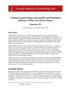
7 These probabilities are also summarized in Figure 1, which displays the predicted probability of low birth weight, along with confidence intervals, as a function of mother s age for those with and without frequent physician visits. Figure 1: Predicted probability of low birth weight as a function of mother s age for those with frequent physician visits (solid line) and those without frequent visits (dashed line). Importantly, the substantive conclusions that an interaction is present and the direction of the interaction will not be affected by the minor discrepancies that come about from using different metrics. They are equally valid techniques for exploring the nature of an interaction in a Logistic Regression model. Both techniques can be implemented in various statistical software packages. If you have any questions regarding implementation or interpretation of these methods, please contact the CSCU Office.

8 Cornell Statistical Consulting Unit Authors: Hongyu Li and Jay Barry